Benchmark: AutoCarver vs. optbinning vs. KBinsDiscretizer
This notebook runs the three binning libraries side-by-side on two public datasets:
German Credit — binary classification, mixed numeric / categorical features, 1,000 rows.
California Housing — regression, all-numeric features, 20,640 rows.
For each library and dataset, we report:
``fit`` and ``transform`` wall-clock (seconds)
Downstream-model score — AUC for binary, R² for regression — using a linear model (logistic regression / ridge) on the one-hot-encoded bin output
``train`` → ``test`` score drop as a coarse proxy for drift sensitivity
All three libraries see the same train + dev data and are evaluated on the same held-out test. AutoCarver uses the dev sample for its built-in robustness veto; optbinning and KBinsDiscretizer don’t have a dev-set concept and so treat the union of train + dev as one pooled training set — which is the comparison practitioners actually run.
This is not an IV / Tschuprow’s T leaderboard. Those metrics structurally favour the library whose objective they are. The downstream-model score is the metric a real scorecard team would use to pick a binner.
Numbers come from a single run on a single machine with a fixed seed; treat them as illustrative, not as authoritative benchmark figures. Re-run on your own data before drawing conclusions.
Setup
[13]:
import time
import warnings

import numpy as np
import pandas as pd
import matplotlib.pyplot as plt
from sklearn.datasets import fetch_california_housing, fetch_openml
from sklearn.linear_model import LogisticRegression, Ridge
from sklearn.metrics import r2_score, roc_auc_score
from sklearn.model_selection import train_test_split
from sklearn.preprocessing import KBinsDiscretizer

from AutoCarver import BinaryCarver, ContinuousCarver, Features
from AutoCarver.discretizers.utils.base_discretizer import DiscretizerConfig

try:
    from optbinning import ContinuousOptimalBinning, OptimalBinning

    HAS_OPTBINNING = True
except ImportError:
    HAS_OPTBINNING = False
    print('optbinning is not installed \u2014 its rows will be skipped.')

SEED = 42
warnings.filterwarnings('ignore')
plt.rcParams['figure.figsize'] = (10, 3.5)
[14]:
def one_hot(df):
    """Treat every bin label as a categorical level and one-hot encode it.

    Lets a linear downstream model consume any of the three libraries' outputs
    uniformly, without us computing WoE per bin.
    """
    return pd.get_dummies(df.astype(str), drop_first=True).astype(float)


def fit_eval_binary(X_train, X_test, y_train, y_test):
    Xtr = one_hot(X_train)
    Xte = one_hot(X_test).reindex(columns=Xtr.columns, fill_value=0.0)
    model = LogisticRegression(max_iter=1000, random_state=SEED).fit(Xtr, y_train)
    return {
        'train_auc': roc_auc_score(y_train, model.predict_proba(Xtr)[:, 1]),
        'test_auc': roc_auc_score(y_test, model.predict_proba(Xte)[:, 1]),
    }


def fit_eval_regression(X_train, X_test, y_train, y_test):
    Xtr = one_hot(X_train)
    Xte = one_hot(X_test).reindex(columns=Xtr.columns, fill_value=0.0)
    model = Ridge(random_state=SEED).fit(Xtr, y_train)
    return {
        'train_r2': r2_score(y_train, model.predict(Xtr)),
        'test_r2': r2_score(y_test, model.predict(Xte)),
    }


def plot_bars(results_df, score_cols, title):
    fig, axes = plt.subplots(1, len(score_cols), figsize=(4 * len(score_cols), 3.5))
    if len(score_cols) == 1:
        axes = [axes]
    for ax, col in zip(axes, score_cols):
        results_df.plot.bar(x='library', y=col, ax=ax, legend=False, color='#4C72B0')
        ax.set_title(col)
        ax.set_xlabel('')
        ax.tick_params(axis='x', rotation=0)
    fig.suptitle(title)
    fig.tight_layout()
    plt.show()
[15]:
from AutoCarver.combinations.binary import CramervCombinations

MAX_N_MOD = 5
MIN_FREQ = 0.05

def bin_with_autocarver(X_train, y_train, X_dev, y_dev, X_test, categoricals, quantitatives, kind):
    Carver = BinaryCarver if kind == 'binary' else ContinuousCarver
    features = Features(categoricals=categoricals, quantitatives=quantitatives)
    config = DiscretizerConfig(verbose=True)  # showing statistics
    combination_evaluator = CramervCombinations() if kind == 'binary' else None
    carver = Carver(features=features, min_freq=MIN_FREQ, max_n_mod=MAX_N_MOD, config=config,combination_evaluator=combination_evaluator)

    t0 = time.perf_counter()
    X_tr = carver.fit_transform(X_train.copy(), y_train, X_dev=X_dev.copy(), y_dev=y_dev)
    fit_t = time.perf_counter() - t0

    X_dv = carver.transform(X_dev.copy())
    t1 = time.perf_counter()
    X_te = carver.transform(X_test.copy())
    transform_t = time.perf_counter() - t1
    return pd.concat([X_tr, X_dv]), X_te, fit_t, transform_t, carver


def bin_with_optbinning(X_train, y_train, X_dev, y_dev, X_test, categoricals, quantitatives, kind):
    Cls = OptimalBinning if kind == 'binary' else ContinuousOptimalBinning
    X_all = pd.concat([X_train, X_dev])
    y_all = pd.concat([y_train, y_dev])
    binners = {}
    train_binned = pd.DataFrame(index=X_all.index)
    test_binned = pd.DataFrame(index=X_test.index)

    t0 = time.perf_counter()
    for col in X_all.columns:
        dtype = 'categorical' if col in categoricals else 'numerical'
        binner = Cls(name=col, dtype=dtype, min_prebin_size=MIN_FREQ/2, max_n_bins=MAX_N_MOD)
        binner.fit(X_all[col].to_numpy(), y_all.to_numpy())
        binners[col] = binner
        train_binned[col] = binner.transform(X_all[col].to_numpy(), metric='bins')
    fit_t = time.perf_counter() - t0

    t1 = time.perf_counter()
    for col, b in binners.items():
        test_binned[col] = b.transform(X_test[col].to_numpy(), metric='bins')
    transform_t = time.perf_counter() - t1
    return train_binned, test_binned, fit_t, transform_t, binners


def bin_with_kbins(X_train, X_dev, X_test, categoricals, quantitatives, n_bins=5):
    X_all = pd.concat([X_train, X_dev])
    num_train = X_all[quantitatives].apply(lambda c: c.fillna(c.median()))
    num_test = X_test[quantitatives].apply(lambda c: c.fillna(c.median()))
    kbd = KBinsDiscretizer(n_bins=n_bins, encode='ordinal', strategy='quantile')

    t0 = time.perf_counter()
    binned_num_train = pd.DataFrame(
        kbd.fit_transform(num_train), columns=quantitatives, index=X_all.index
    )
    fit_t = time.perf_counter() - t0

    t1 = time.perf_counter()
    binned_num_test = pd.DataFrame(
        kbd.transform(num_test), columns=quantitatives, index=X_test.index
    )
    transform_t = time.perf_counter() - t1

    # KBins has no opinion on categoricals — pass them through as labels
    train = pd.concat([binned_num_train, X_all[categoricals].astype(str)], axis=1)
    test = pd.concat([binned_num_test, X_test[categoricals].astype(str)], axis=1)
    return train, test, fit_t, transform_t, kbd
Binary classification — German Credit
20 features (numeric + categorical), 1,000 rows, target = class == 'bad'. Train / dev / test split = 60 / 20 / 20 %.
[16]:
credit = fetch_openml(data_id=31, as_frame=True)
df = credit.frame.copy()

y_binary = (df['class'] == 'bad').astype(int)
X_binary = df.drop(columns=['class'])

X_train, X_rest, y_train, y_rest = train_test_split(
    X_binary, y_binary, test_size=0.4, random_state=SEED, stratify=y_binary,
)
X_dev, X_test, y_dev, y_test = train_test_split(
    X_rest, y_rest, test_size=0.5, random_state=SEED, stratify=y_rest,
)

categoricals = [c for c in X_binary.columns if X_binary[c].dtype == object or isinstance(X_binary[c].dtype, pd.CategoricalDtype)]
quantitatives = [c for c in X_binary.columns if c not in categoricals]

print(f'train={len(X_train)}, dev={len(X_dev)}, test={len(X_test)}')
print(f'categoricals={len(categoricals)}, quantitatives={len(quantitatives)}')
print(f'bad rate (train)={y_train.mean():.3f}, (test)={y_test.mean():.3f}')
train=600, dev=200, test=200
categoricals=13, quantitatives=7
bad rate (train)=0.300, (test)=0.300
[17]:
y_train_full = pd.concat([y_train, y_dev])

runs = [(
    'AutoCarver',
    lambda: bin_with_autocarver(X_train, y_train, X_dev, y_dev, X_test, categoricals, quantitatives, 'binary'),
)]
if HAS_OPTBINNING:
    runs.append((
        'optbinning',
        lambda: bin_with_optbinning(X_train, y_train, X_dev, y_dev, X_test, categoricals, quantitatives, 'binary'),
    ))
runs.append((
    'KBinsDiscretizer',
    lambda: bin_with_kbins(X_train, X_dev, X_test, categoricals, quantitatives),
))

rows = []
for name, run in runs:
    X_tr, X_te, fit_t, transform_t, carver = run()
    scores = fit_eval_binary(X_tr, X_te, y_train_full, y_test)
    rows.append({
        'library': name,
        'fit_s': round(fit_t, 3),
        'transform_s': round(transform_t, 4),
        'train_auc': round(scores['train_auc'], 4),
        'test_auc': round(scores['test_auc'], 4),
        'auc_drop': round(scores['train_auc'] - scores['test_auc'], 4),
    })

binary_results = pd.DataFrame(rows)
binary_results
------
--- [QuantitativeDiscretizer] Fit Features(['duration', 'credit_amount', 'installment_commitment', 'residence_since', 'age', 'existing_credits', 'num_dependents'])
 - [ContinuousDiscretizer] Fit Features(['duration', 'credit_amount', 'installment_commitment', 'residence_since', 'age', 'existing_credits', 'num_dependents'])
 - [OrdinalDiscretizer] Fit Features(['duration', 'installment_commitment', 'residence_since', 'existing_credits', 'num_dependents'])
------

------
--- [QualitativeDiscretizer] Fit Features(['checking_status', 'credit_history', 'purpose', 'savings_status', 'employment', 'personal_status', 'other_parties', 'property_magnitude', 'other_payment_plans', 'housing', 'job', 'own_telephone', 'foreign_worker'])
 - [CategoricalDiscretizer] Fit Features(['checking_status', 'credit_history', 'purpose', 'savings_status', 'employment', 'personal_status', 'other_parties', 'property_magnitude', 'other_payment_plans', 'housing', 'job', 'own_telephone', 'foreign_worker'])
------

---------
------ [BinaryCarver] Fit Features(['checking_status', 'credit_history', 'purpose', 'savings_status', 'employment', 'personal_status', 'other_parties', 'property_magnitude', 'other_payment_plans', 'housing', 'job', 'own_telephone', 'foreign_worker', 'duration', 'credit_amount', 'installment_commitment', 'residence_since', 'age', 'existing_credits', 'num_dependents'])
--- [BinaryCarver] Fit Categorical('checking_status') (1/20)
 [BinaryCarver] Raw distribution
| target_mean | frequency | count | |
|---|---|---|---|
| no checking | 0.1317 | 0.4050 | 243 |
| >=200 | 0.2778 | 0.0600 | 36 |
| 0<=X<200 | 0.3896 | 0.2567 | 154 |
| <0 | 0.4671 | 0.2783 | 167 |
| target_mean | frequency | count |
|---|---|---|
| 0.0694 | 0.3600 | 72 |
| 0.0833 | 0.0600 | 12 |
| 0.3710 | 0.3100 | 62 |
| 0.5741 | 0.2700 | 54 |
[BinaryCarver] Carved distribution
| target_mean | frequency | count | |
|---|---|---|---|
| no checking | 0.1317 | 0.4050 | 243 |
| >=200 | 0.2778 | 0.0600 | 36 |
| 0<=X<200 | 0.3896 | 0.2567 | 154 |
| <0 | 0.4671 | 0.2783 | 167 |
| target_mean | frequency | count |
|---|---|---|
| 0.0694 | 0.3600 | 72 |
| 0.0833 | 0.0600 | 12 |
| 0.3710 | 0.3100 | 62 |
| 0.5741 | 0.2700 | 54 |
--- [BinaryCarver] Fit Categorical('credit_history') (2/20)
 [BinaryCarver] Raw distribution
| target_mean | frequency | count | |
|---|---|---|---|
| critical/other existing credit | 0.1676 | 0.2883 | 173 |
| existing paid | 0.3185 | 0.5233 | 314 |
| delayed previously | 0.3621 | 0.0967 | 58 |
| all paid | 0.5455 | 0.0550 | 33 |
| no credits/all paid | 0.5455 | 0.0367 | 22 |
| target_mean | frequency | count |
|---|---|---|
| 0.2241 | 0.2900 | 58 |
| 0.2703 | 0.5550 | 111 |
| 0.3571 | 0.0700 | 14 |
| 0.7273 | 0.0550 | 11 |
| 0.6667 | 0.0300 | 6 |
[BinaryCarver] Carved distribution
| target_mean | frequency | count | |
|---|---|---|---|
| critical/other existing credit | 0.1676 | 0.2883 | 173 |
| existing paid | 0.3185 | 0.5233 | 314 |
| delayed previously | 0.3621 | 0.0967 | 58 |
| all paid, no credits/all paid | 0.5455 | 0.0917 | 55 |
| target_mean | frequency | count |
|---|---|---|
| 0.2241 | 0.2900 | 58 |
| 0.2703 | 0.5550 | 111 |
| 0.3571 | 0.0700 | 14 |
| 0.7059 | 0.0850 | 17 |
--- [BinaryCarver] Fit Categorical('purpose') (3/20)
 [BinaryCarver] Raw distribution
| target_mean | frequency | count | |
|---|---|---|---|
| used car | 0.1875 | 0.1067 | 64 |
| other, retraining | 0.2222 | 0.0150 | 9 |
| radio/tv | 0.2303 | 0.2750 | 165 |
| domestic appliance | 0.3000 | 0.0167 | 10 |
| furniture/equipment | 0.3333 | 0.1700 | 102 |
| new car | 0.3401 | 0.2450 | 147 |
| business | 0.3729 | 0.0983 | 59 |
| repairs | 0.3750 | 0.0267 | 16 |
| education | 0.4643 | 0.0467 | 28 |
| target_mean | frequency | count |
|---|---|---|
| 0.1250 | 0.0800 | 16 |
| 0.3000 | 0.0500 | 10 |
| 0.2295 | 0.3050 | 61 |
| 0.0000 | 0.0050 | 1 |
| 0.3235 | 0.1700 | 34 |
| 0.4222 | 0.2250 | 45 |
| 0.2778 | 0.0900 | 18 |
| 0.0000 | 0.0100 | 2 |
| 0.4615 | 0.0650 | 13 |
[BinaryCarver] Carved distribution
| target_mean | frequency | count | |
|---|---|---|---|
| used car | 0.1875 | 0.1067 | 64 |
| radio/tv, other, retraining | 0.2299 | 0.2900 | 174 |
| furniture/equipment, domestic appliance | 0.3304 | 0.1867 | 112 |
| new car, business, repairs | 0.3514 | 0.3700 | 222 |
| education | 0.4643 | 0.0467 | 28 |
| target_mean | frequency | count |
|---|---|---|
| 0.1250 | 0.0800 | 16 |
| 0.2394 | 0.3550 | 71 |
| 0.3143 | 0.1750 | 35 |
| 0.3692 | 0.3250 | 65 |
| 0.4615 | 0.0650 | 13 |
--- [BinaryCarver] Fit Categorical('savings_status') (4/20)
 [BinaryCarver] Raw distribution
| target_mean | frequency | count | |
|---|---|---|---|
| >=1000 | 0.0667 | 0.0500 | 30 |
| 500<=X<1000 | 0.1622 | 0.0617 | 37 |
| no known savings | 0.1714 | 0.1750 | 105 |
| 100<=X<500 | 0.3333 | 0.1150 | 69 |
| <100 | 0.3649 | 0.5983 | 359 |
| target_mean | frequency | count |
|---|---|---|
| 0.3333 | 0.0300 | 6 |
| 0.1250 | 0.0800 | 16 |
| 0.1667 | 0.1800 | 36 |
| 0.3889 | 0.0900 | 18 |
| 0.3468 | 0.6200 | 124 |
[BinaryCarver] Carved distribution
| target_mean | frequency | count | |
|---|---|---|---|
| no known savings, >=1000, 500<=X<1000 | 0.1512 | 0.2867 | 172 |
| <100, 100<=X<500 | 0.3598 | 0.7133 | 428 |
| target_mean | frequency | count |
|---|---|---|
| 0.1724 | 0.2900 | 58 |
| 0.3521 | 0.7100 | 142 |
--- [BinaryCarver] Fit Categorical('employment') (5/20)
 [BinaryCarver] Raw distribution
| target_mean | frequency | count | |
|---|---|---|---|
| 4<=X<7 | 0.1935 | 0.1550 | 93 |
| >=7 | 0.2516 | 0.2650 | 159 |
| 1<=X<4 | 0.2911 | 0.3550 | 213 |
| <1 | 0.4272 | 0.1717 | 103 |
| unemployed | 0.5000 | 0.0533 | 32 |
| target_mean | frequency | count |
|---|---|---|
| 0.2632 | 0.1900 | 38 |
| 0.2600 | 0.2500 | 50 |
| 0.3621 | 0.2900 | 58 |
| 0.3333 | 0.1800 | 36 |
| 0.2222 | 0.0900 | 18 |
[BinaryCarver] Carved distribution
| target_mean | frequency | count | |
|---|---|---|---|
| >=7, 4<=X<7 | 0.2302 | 0.4200 | 252 |
| unemployed, 1<=X<4, <1 | 0.3506 | 0.5800 | 348 |
| target_mean | frequency | count |
|---|---|---|
| 0.2614 | 0.4400 | 88 |
| 0.3304 | 0.5600 | 112 |
--- [BinaryCarver] Fit Categorical('personal_status') (6/20)
 [BinaryCarver] Raw distribution
| target_mean | frequency | count | |
|---|---|---|---|
| male single | 0.2679 | 0.5600 | 336 |
| male mar/wid | 0.2778 | 0.0900 | 54 |
| female div/dep/mar | 0.3559 | 0.2950 | 177 |
| male div/sep | 0.3636 | 0.0550 | 33 |
| target_mean | frequency | count |
|---|---|---|
| 0.2830 | 0.5300 | 106 |
| 0.2381 | 0.1050 | 21 |
| 0.3385 | 0.3250 | 65 |
| 0.3750 | 0.0400 | 8 |
[BinaryCarver] Carved distribution
| target_mean | frequency | count | |
|---|---|---|---|
| male single, male mar/wid | 0.2692 | 0.6500 | 390 |
| female div/dep/mar | 0.3559 | 0.2950 | 177 |
| male div/sep | 0.3636 | 0.0550 | 33 |
| target_mean | frequency | count |
|---|---|---|
| 0.2756 | 0.6350 | 127 |
| 0.3385 | 0.3250 | 65 |
| 0.3750 | 0.0400 | 8 |
--- [BinaryCarver] Fit Categorical('other_parties') (7/20)
 [BinaryCarver] Raw distribution
| target_mean | frequency | count | |
|---|---|---|---|
| guarantor | 0.1786 | 0.0467 | 28 |
| none | 0.2996 | 0.9067 | 544 |
| co applicant | 0.4286 | 0.0467 | 28 |
| target_mean | frequency | count |
|---|---|---|
| 0.2500 | 0.0400 | 8 |
| 0.2989 | 0.9200 | 184 |
| 0.3750 | 0.0400 | 8 |
[BinaryCarver] Carved distribution
| target_mean | frequency | count | |
|---|---|---|---|
| guarantor | 0.1786 | 0.0467 | 28 |
| none | 0.2996 | 0.9067 | 544 |
| co applicant | 0.4286 | 0.0467 | 28 |
| target_mean | frequency | count |
|---|---|---|
| 0.2500 | 0.0400 | 8 |
| 0.2989 | 0.9200 | 184 |
| 0.3750 | 0.0400 | 8 |
--- [BinaryCarver] Fit Categorical('property_magnitude') (8/20)
 [BinaryCarver] Raw distribution
| target_mean | frequency | count | |
|---|---|---|---|
| real estate | 0.2130 | 0.2817 | 169 |
| life insurance | 0.3125 | 0.2133 | 128 |
| car | 0.3143 | 0.3500 | 210 |
| no known property | 0.4086 | 0.1550 | 93 |
| target_mean | frequency | count |
|---|---|---|
| 0.2182 | 0.2750 | 55 |
| 0.2600 | 0.2500 | 50 |
| 0.3281 | 0.3200 | 64 |
| 0.4516 | 0.1550 | 31 |
[BinaryCarver] Carved distribution
| target_mean | frequency | count | |
|---|---|---|---|
| real estate | 0.2130 | 0.2817 | 169 |
| life insurance | 0.3125 | 0.2133 | 128 |
| car | 0.3143 | 0.3500 | 210 |
| no known property | 0.4086 | 0.1550 | 93 |
| target_mean | frequency | count |
|---|---|---|
| 0.2182 | 0.2750 | 55 |
| 0.2600 | 0.2500 | 50 |
| 0.3281 | 0.3200 | 64 |
| 0.4516 | 0.1550 | 31 |
--- [BinaryCarver] Fit Categorical('other_payment_plans') (9/20)
 [BinaryCarver] Raw distribution
| target_mean | frequency | count | |
|---|---|---|---|
| none | 0.2619 | 0.8083 | 485 |
| stores | 0.4375 | 0.0533 | 32 |
| bank | 0.4699 | 0.1383 | 83 |
| target_mean | frequency | count |
|---|---|---|
| 0.2866 | 0.8200 | 164 |
| 0.4444 | 0.0450 | 9 |
| 0.3333 | 0.1350 | 27 |
[BinaryCarver] Carved distribution
| target_mean | frequency | count | |
|---|---|---|---|
| none | 0.2619 | 0.8083 | 485 |
| bank, stores | 0.4609 | 0.1917 | 115 |
| target_mean | frequency | count |
|---|---|---|
| 0.2866 | 0.8200 | 164 |
| 0.3611 | 0.1800 | 36 |
--- [BinaryCarver] Fit Categorical('housing') (10/20)
 [BinaryCarver] Raw distribution
| target_mean | frequency | count | |
|---|---|---|---|
| own | 0.2558 | 0.7233 | 434 |
| for free | 0.3750 | 0.1067 | 64 |
| rent | 0.4412 | 0.1700 | 102 |
| target_mean | frequency | count |
|---|---|---|
| 0.2857 | 0.7350 | 147 |
| 0.4348 | 0.1150 | 23 |
| 0.2667 | 0.1500 | 30 |
[BinaryCarver] Carved distribution
| target_mean | frequency | count | |
|---|---|---|---|
| own | 0.2558 | 0.7233 | 434 |
| for free, rent | 0.4157 | 0.2767 | 166 |
| target_mean | frequency | count |
|---|---|---|
| 0.2857 | 0.7350 | 147 |
| 0.3396 | 0.2650 | 53 |
--- [BinaryCarver] Fit Categorical('job') (11/20)
 [BinaryCarver] Raw distribution
| target_mean | frequency | count | |
|---|---|---|---|
| skilled | 0.2898 | 0.6383 | 383 |
| unskilled resident | 0.2966 | 0.1967 | 118 |
| high qualif/self emp/mgmt | 0.3258 | 0.1483 | 89 |
| unemp/unskilled non res | 0.5000 | 0.0167 | 10 |
| target_mean | frequency | count |
|---|---|---|
| 0.2541 | 0.6100 | 122 |
| 0.3171 | 0.2050 | 41 |
| 0.4839 | 0.1550 | 31 |
| 0.1667 | 0.0300 | 6 |
[BinaryCarver] Carved distribution
| target_mean | frequency | count | |
|---|---|---|---|
| skilled | 0.2898 | 0.6383 | 383 |
| unskilled resident | 0.2966 | 0.1967 | 118 |
| high qualif/self emp/mgmt, unemp/unskilled non res | 0.3434 | 0.1650 | 99 |
| target_mean | frequency | count |
|---|---|---|
| 0.2541 | 0.6100 | 122 |
| 0.3171 | 0.2050 | 41 |
| 0.4324 | 0.1850 | 37 |
--- [BinaryCarver] Fit Categorical('own_telephone') (12/20)
 [BinaryCarver] Raw distribution
| target_mean | frequency | count | |
|---|---|---|---|
| yes | 0.2645 | 0.4033 | 242 |
| none | 0.3240 | 0.5967 | 358 |
| target_mean | frequency | count |
|---|---|---|
| 0.3125 | 0.4000 | 80 |
| 0.2917 | 0.6000 | 120 |
WARNING: No robust combination for Categorical('own_telephone'). Consider increasing the size of X_dev or dropping the feature (X not representative of X_dev for this feature).
--- [BinaryCarver] Fit Categorical('foreign_worker') (13/20)
 [BinaryCarver] Raw distribution
| target_mean | frequency | count | |
|---|---|---|---|
| no | 0.0435 | 0.0383 | 23 |
| yes | 0.3102 | 0.9617 | 577 |
| target_mean | frequency | count |
|---|---|---|
| 0.3333 | 0.0300 | 6 |
| 0.2990 | 0.9700 | 194 |
WARNING: No robust combination for Categorical('foreign_worker'). Consider increasing the size of X_dev or dropping the feature (X not representative of X_dev for this feature).
--- [BinaryCarver] Fit Quantitative('duration') (14/20)
 [BinaryCarver] Raw distribution
| target_mean | frequency | count | |
|---|---|---|---|
| x <= 8.00e+00 | 0.0980 | 0.0850 | 51 |
| 8.00e+00 < x <= 9.00e+00 | 0.2333 | 0.0500 | 30 |
| 9.00e+00 < x <= 1.10e+01 | 0.0870 | 0.0383 | 23 |
| 1.10e+01 < x <= 1.20e+01 | 0.2883 | 0.1850 | 111 |
| 1.20e+01 < x <= 1.50e+01 | 0.2273 | 0.0733 | 44 |
| 1.50e+01 < x <= 1.80e+01 | 0.3692 | 0.1083 | 65 |
| 1.80e+01 < x <= 2.20e+01 | 0.2381 | 0.0350 | 21 |
| 2.20e+01 < x <= 2.40e+01 | 0.3333 | 0.1950 | 117 |
| 2.40e+01 < x <= 2.80e+01 | 0.2222 | 0.0150 | 9 |
| 2.80e+01 < x <= 3.30e+01 | 0.3846 | 0.0433 | 26 |
| 3.30e+01 < x <= 3.60e+01 | 0.4727 | 0.0917 | 55 |
| 3.60e+01 < x <= 4.70e+01 | 0.2667 | 0.0250 | 15 |
| 4.70e+01 < x | 0.4242 | 0.0550 | 33 |
| target_mean | frequency | count |
|---|---|---|
| 0.1000 | 0.1000 | 20 |
| 0.3077 | 0.0650 | 13 |
| 0.0000 | 0.0400 | 8 |
| 0.2432 | 0.1850 | 37 |
| 0.0714 | 0.0700 | 14 |
| 0.3043 | 0.1150 | 23 |
| 0.4444 | 0.0450 | 9 |
| 0.3548 | 0.1550 | 31 |
| 0.7500 | 0.0200 | 4 |
| 0.4286 | 0.0350 | 7 |
| 0.3529 | 0.0850 | 17 |
| 0.6667 | 0.0150 | 3 |
| 0.5714 | 0.0700 | 14 |
[BinaryCarver] Carved distribution
| target_mean | frequency | count | |
|---|---|---|---|
| x <= 8.00e+00 | 0.0980 | 0.0850 | 51 |
| 8.00e+00 < x <= 1.10e+01 | 0.1698 | 0.0883 | 53 |
| 1.10e+01 < x <= 1.50e+01 | 0.2710 | 0.2583 | 155 |
| 1.50e+01 < x <= 2.80e+01 | 0.3302 | 0.3533 | 212 |
| 2.80e+01 < x | 0.4186 | 0.2150 | 129 |
| target_mean | frequency | count |
|---|---|---|
| 0.1000 | 0.1000 | 20 |
| 0.1905 | 0.1050 | 21 |
| 0.1961 | 0.2550 | 51 |
| 0.3731 | 0.3350 | 67 |
| 0.4634 | 0.2050 | 41 |
--- [BinaryCarver] Fit Quantitative('credit_amount') (15/20)
 [BinaryCarver] Raw distribution
| target_mean | frequency | count | |
|---|---|---|---|
| x <= 6.18e+02 | 0.2000 | 0.0250 | 15 |
| 6.18e+02 < x <= 7.08e+02 | 0.4000 | 0.0250 | 15 |
| 7.08e+02 < x <= 7.97e+02 | 0.3333 | 0.0250 | 15 |
| 7.97e+02 < x <= 9.09e+02 | 0.4000 | 0.0250 | 15 |
| 9.09e+02 < x <= 1.03e+03 | 0.4000 | 0.0250 | 15 |
| 1.03e+03 < x <= 1.16e+03 | 0.2000 | 0.0250 | 15 |
| 1.16e+03 < x <= 1.21e+03 | 0.2667 | 0.0250 | 15 |
| 1.21e+03 < x <= 1.26e+03 | 0.2000 | 0.0250 | 15 |
| 1.26e+03 < x <= 1.31e+03 | 0.3333 | 0.0250 | 15 |
| 1.31e+03 < x <= 1.37e+03 | 0.4667 | 0.0250 | 15 |
| 1.37e+03 < x <= 1.41e+03 | 0.1250 | 0.0267 | 16 |
| 1.41e+03 < x <= 1.47e+03 | 0.1429 | 0.0233 | 14 |
| 1.47e+03 < x <= 1.53e+03 | 0.2667 | 0.0250 | 15 |
| 1.53e+03 < x <= 1.60e+03 | 0.2000 | 0.0250 | 15 |
| 1.60e+03 < x <= 1.82e+03 | 0.2000 | 0.0250 | 15 |
| 1.82e+03 < x <= 1.92e+03 | 0.5000 | 0.0267 | 16 |
| 1.92e+03 < x <= 1.98e+03 | 0.2857 | 0.0233 | 14 |
| 1.98e+03 < x <= 2.12e+03 | 0.3333 | 0.0250 | 15 |
| 2.12e+03 < x <= 2.21e+03 | 0.2667 | 0.0250 | 15 |
| 2.21e+03 < x <= 2.30e+03 | 0.2667 | 0.0250 | 15 |
| 2.30e+03 < x <= 2.38e+03 | 0.2000 | 0.0250 | 15 |
| 2.38e+03 < x <= 2.48e+03 | 0.4000 | 0.0250 | 15 |
| 2.48e+03 < x <= 2.62e+03 | 0.2667 | 0.0250 | 15 |
| 2.62e+03 < x <= 2.75e+03 | 0.3333 | 0.0250 | 15 |
| 2.75e+03 < x <= 2.92e+03 | 0.2000 | 0.0250 | 15 |
| 2.92e+03 < x <= 3.07e+03 | 0.2000 | 0.0250 | 15 |
| 3.07e+03 < x <= 3.35e+03 | 0.4000 | 0.0250 | 15 |
| 3.35e+03 < x <= 3.51e+03 | 0.1333 | 0.0250 | 15 |
| 3.51e+03 < x <= 3.63e+03 | 0.1333 | 0.0250 | 15 |
| 3.63e+03 < x <= 3.91e+03 | 0.0667 | 0.0250 | 15 |
| 3.91e+03 < x <= 4.24e+03 | 0.4667 | 0.0250 | 15 |
| 4.24e+03 < x <= 4.66e+03 | 0.4000 | 0.0250 | 15 |
| 4.66e+03 < x <= 5.08e+03 | 0.4667 | 0.0250 | 15 |
| 5.08e+03 < x <= 5.80e+03 | 0.2000 | 0.0250 | 15 |
| 5.80e+03 < x <= 6.36e+03 | 0.2667 | 0.0250 | 15 |
| 6.36e+03 < x <= 6.85e+03 | 0.4667 | 0.0250 | 15 |
| 6.85e+03 < x <= 7.48e+03 | 0.2000 | 0.0250 | 15 |
| 7.48e+03 < x <= 8.23e+03 | 0.4667 | 0.0250 | 15 |
| 8.23e+03 < x <= 9.57e+03 | 0.4000 | 0.0250 | 15 |
| 9.57e+03 < x | 0.5333 | 0.0250 | 15 |
| target_mean | frequency | count |
|---|---|---|
| 0.2000 | 0.0250 | 5 |
| 0.5000 | 0.0200 | 4 |
| 0.5000 | 0.0300 | 6 |
| 0.0000 | 0.0100 | 2 |
| 0.3333 | 0.0300 | 6 |
| 0.1429 | 0.0350 | 7 |
| 0.5000 | 0.0100 | 2 |
| 0.3333 | 0.0600 | 12 |
| 0.0000 | 0.0100 | 2 |
| 0.2857 | 0.0350 | 7 |
| 0.0000 | 0.0150 | 3 |
| 0.3333 | 0.0300 | 6 |
| 0.2500 | 0.0200 | 4 |
| 0.0000 | 0.0150 | 3 |
| 0.3333 | 0.0300 | 6 |
| 0.2857 | 0.0350 | 7 |
| 0.2500 | 0.0200 | 4 |
| 0.0000 | 0.0400 | 8 |
| 0.5000 | 0.0100 | 2 |
| 0.5000 | 0.0100 | 2 |
| 0.0000 | 0.0150 | 3 |
| 0.0000 | 0.0050 | 1 |
| 0.6667 | 0.0150 | 3 |
| 0.0000 | 0.0200 | 4 |
| 0.0000 | 0.0200 | 4 |
| 0.3333 | 0.0150 | 3 |
| 0.2000 | 0.0500 | 10 |
| 0.5000 | 0.0400 | 8 |
| 0.0000 | 0.0300 | 6 |
| 0.1000 | 0.0500 | 10 |
| 0.2500 | 0.0200 | 4 |
| 0.8000 | 0.0250 | 5 |
| 0.3333 | 0.0150 | 3 |
| 0.4000 | 0.0250 | 5 |
| 0.2857 | 0.0350 | 7 |
| 0.0000 | 0.0200 | 4 |
| 0.6667 | 0.0150 | 3 |
| 0.6667 | 0.0150 | 3 |
| 0.6667 | 0.0150 | 3 |
| 0.6154 | 0.0650 | 13 |
[BinaryCarver] Carved distribution
| target_mean | frequency | count | |
|---|---|---|---|
| x <= 1.03e+03 | 0.3467 | 0.1250 | 75 |
| 1.03e+03 < x <= 3.35e+03 | 0.2758 | 0.5500 | 330 |
| 3.35e+03 < x <= 3.91e+03 | 0.1111 | 0.0750 | 45 |
| 3.91e+03 < x <= 7.48e+03 | 0.3524 | 0.1750 | 105 |
| 7.48e+03 < x | 0.4667 | 0.0750 | 45 |
| target_mean | frequency | count |
|---|---|---|
| 0.3478 | 0.1150 | 23 |
| 0.2233 | 0.5150 | 103 |
| 0.2083 | 0.1200 | 24 |
| 0.3871 | 0.1550 | 31 |
| 0.6316 | 0.0950 | 19 |
--- [BinaryCarver] Fit Quantitative('installment_commitment') (16/20)
 [BinaryCarver] Raw distribution
| target_mean | frequency | count | |
|---|---|---|---|
| x <= 1.00e+00 | 0.2436 | 0.1300 | 78 |
| 1.00e+00 < x <= 2.00e+00 | 0.2606 | 0.2367 | 142 |
| 2.00e+00 < x <= 3.00e+00 | 0.2979 | 0.1567 | 94 |
| 3.00e+00 < x | 0.3357 | 0.4767 | 286 |
| target_mean | frequency | count |
|---|---|---|
| 0.1071 | 0.1400 | 28 |
| 0.2667 | 0.2250 | 45 |
| 0.2414 | 0.1450 | 29 |
| 0.3878 | 0.4900 | 98 |
[BinaryCarver] Carved distribution
| target_mean | frequency | count | |
|---|---|---|---|
| x <= 2.00e+00 | 0.2545 | 0.3667 | 220 |
| 2.00e+00 < x <= 3.00e+00 | 0.2979 | 0.1567 | 94 |
| 3.00e+00 < x | 0.3357 | 0.4767 | 286 |
| target_mean | frequency | count |
|---|---|---|
| 0.2055 | 0.3650 | 73 |
| 0.2414 | 0.1450 | 29 |
| 0.3878 | 0.4900 | 98 |
--- [BinaryCarver] Fit Quantitative('residence_since') (17/20)
 [BinaryCarver] Raw distribution
| target_mean | frequency | count | |
|---|---|---|---|
| x <= 1.00e+00 | 0.3117 | 0.1283 | 77 |
| 1.00e+00 < x <= 2.00e+00 | 0.2905 | 0.2983 | 179 |
| 2.00e+00 < x <= 3.00e+00 | 0.3000 | 0.1667 | 100 |
| 3.00e+00 < x | 0.3033 | 0.4067 | 244 |
| target_mean | frequency | count |
|---|---|---|
| 0.2174 | 0.1150 | 23 |
| 0.3529 | 0.3400 | 68 |
| 0.3333 | 0.1500 | 30 |
| 0.2658 | 0.3950 | 79 |
WARNING: No robust combination for Quantitative('residence_since'). Consider increasing the size of X_dev or dropping the feature (X not representative of X_dev for this feature).
--- [BinaryCarver] Fit Quantitative('age') (18/20)
 [BinaryCarver] Raw distribution
| target_mean | frequency | count | |
|---|---|---|---|
| x <= 2.10e+01 | 0.4000 | 0.0250 | 15 |
| 2.10e+01 < x <= 2.20e+01 | 0.3684 | 0.0317 | 19 |
| 2.20e+01 < x <= 2.30e+01 | 0.4500 | 0.0333 | 20 |
| 2.30e+01 < x <= 2.40e+01 | 0.3333 | 0.0350 | 21 |
| 2.40e+01 < x <= 2.50e+01 | 0.5161 | 0.0517 | 31 |
| 2.50e+01 < x <= 2.60e+01 | 0.2500 | 0.0467 | 28 |
| 2.60e+01 < x <= 2.70e+01 | 0.2258 | 0.0517 | 31 |
| 2.70e+01 < x <= 2.80e+01 | 0.4091 | 0.0367 | 22 |
| 2.80e+01 < x <= 2.90e+01 | 0.3913 | 0.0383 | 23 |
| 2.90e+01 < x <= 3.00e+01 | 0.2143 | 0.0467 | 28 |
| 3.00e+01 < x <= 3.10e+01 | 0.2308 | 0.0433 | 26 |
| 3.10e+01 < x <= 3.20e+01 | 0.2500 | 0.0333 | 20 |
| 3.20e+01 < x <= 3.30e+01 | 0.3636 | 0.0367 | 22 |
| 3.30e+01 < x <= 3.40e+01 | 0.3636 | 0.0367 | 22 |
| 3.40e+01 < x <= 3.50e+01 | 0.1724 | 0.0483 | 29 |
| 3.50e+01 < x <= 3.60e+01 | 0.2083 | 0.0400 | 24 |
| 3.60e+01 < x <= 3.70e+01 | 0.3333 | 0.0250 | 15 |
| 3.70e+01 < x <= 3.80e+01 | 0.1875 | 0.0267 | 16 |
| 3.80e+01 < x <= 3.90e+01 | 0.2941 | 0.0283 | 17 |
| 3.90e+01 < x <= 4.10e+01 | 0.3182 | 0.0367 | 22 |
| 4.10e+01 < x <= 4.20e+01 | 0.2727 | 0.0183 | 11 |
| 4.20e+01 < x <= 4.40e+01 | 0.1905 | 0.0350 | 21 |
| 4.40e+01 < x <= 4.60e+01 | 0.2632 | 0.0317 | 19 |
| 4.60e+01 < x <= 4.70e+01 | 0.4000 | 0.0167 | 10 |
| 4.70e+01 < x <= 4.90e+01 | 0.1429 | 0.0233 | 14 |
| 4.90e+01 < x <= 5.10e+01 | 0.1429 | 0.0233 | 14 |
| 5.10e+01 < x <= 5.40e+01 | 0.2941 | 0.0283 | 17 |
| 5.40e+01 < x <= 5.70e+01 | 0.3333 | 0.0200 | 12 |
| 5.70e+01 < x <= 6.30e+01 | 0.4375 | 0.0267 | 16 |
| 6.30e+01 < x | 0.2667 | 0.0250 | 15 |
| target_mean | frequency | count |
|---|---|---|
| 0.3333 | 0.0300 | 6 |
| 0.5000 | 0.0200 | 4 |
| 0.3333 | 0.0750 | 15 |
| 0.6364 | 0.0550 | 11 |
| 0.3333 | 0.0150 | 3 |
| 0.3333 | 0.0600 | 12 |
| 0.1538 | 0.0650 | 13 |
| 0.1429 | 0.0350 | 7 |
| 0.4000 | 0.0250 | 5 |
| 0.5000 | 0.0500 | 10 |
| 0.3333 | 0.0300 | 6 |
| 0.2000 | 0.0250 | 5 |
| 0.3750 | 0.0400 | 8 |
| 0.3333 | 0.0150 | 3 |
| 0.2500 | 0.0200 | 4 |
| 0.1429 | 0.0350 | 7 |
| 0.2500 | 0.0400 | 8 |
| 0.2500 | 0.0200 | 4 |
| 0.0000 | 0.0050 | 1 |
| 0.2308 | 0.0650 | 13 |
| 0.6000 | 0.0250 | 5 |
| 0.3333 | 0.0300 | 6 |
| 0.1250 | 0.0400 | 8 |
| 0.0000 | 0.0200 | 4 |
| 0.2000 | 0.0250 | 5 |
| 0.5000 | 0.0100 | 2 |
| 0.6000 | 0.0250 | 5 |
| 0.2500 | 0.0200 | 4 |
| 0.2500 | 0.0400 | 8 |
| 0.0000 | 0.0400 | 8 |
[BinaryCarver] Carved distribution
| target_mean | frequency | count | |
|---|---|---|---|
| x <= 2.50e+01 | 0.4245 | 0.1767 | 106 |
| 2.50e+01 < x <= 3.20e+01 | 0.2753 | 0.2967 | 178 |
| 3.20e+01 < x <= 3.40e+01 | 0.3636 | 0.0733 | 44 |
| 3.40e+01 < x <= 3.60e+01 | 0.1887 | 0.0883 | 53 |
| 3.60e+01 < x | 0.2740 | 0.3650 | 219 |
| target_mean | frequency | count |
|---|---|---|
| 0.4359 | 0.1950 | 39 |
| 0.2931 | 0.2900 | 58 |
| 0.3636 | 0.0550 | 11 |
| 0.1818 | 0.0550 | 11 |
| 0.2469 | 0.4050 | 81 |
--- [BinaryCarver] Fit Quantitative('existing_credits') (19/20)
 [BinaryCarver] Raw distribution
| target_mean | frequency | count | |
|---|---|---|---|
| x <= 1.00e+00 | 0.3061 | 0.6317 | 379 |
| 1.00e+00 < x <= 2.00e+00 | 0.2899 | 0.3450 | 207 |
| 2.00e+00 < x | 0.2857 | 0.0233 | 14 |
| target_mean | frequency | count |
|---|---|---|
| 0.3000 | 0.6500 | 130 |
| 0.3016 | 0.3150 | 63 |
| 0.2857 | 0.0350 | 7 |
WARNING: No robust combination for Quantitative('existing_credits'). Consider increasing the size of X_dev or dropping the feature (X not representative of X_dev for this feature).
--- [BinaryCarver] Fit Quantitative('num_dependents') (20/20)
 [BinaryCarver] Raw distribution
| target_mean | frequency | count | |
|---|---|---|---|
| x <= 1.0e+00 | 0.2984 | 0.8433 | 506 |
| 1.0e+00 < x | 0.3085 | 0.1567 | 94 |
| target_mean | frequency | count |
|---|---|---|
| 0.3000 | 0.8500 | 170 |
| 0.3000 | 0.1500 | 30 |
WARNING: No robust combination for Quantitative('num_dependents'). Consider increasing the size of X_dev or dropping the feature (X not representative of X_dev for this feature).
[17]:
| library | fit_s | transform_s | train_auc | test_auc | auc_drop | |
|---|---|---|---|---|---|---|
| 0 | AutoCarver | 1.948 | 0.0115 | 0.8474 | 0.8118 | 0.0356 |
| 1 | optbinning | 1.025 | 0.0141 | 0.8523 | 0.7931 | 0.0592 |
| 2 | KBinsDiscretizer | 0.002 | 0.0009 | 0.8401 | 0.7943 | 0.0458 |
[18]:
plot_bars(binary_results, ['fit_s', 'test_auc', 'auc_drop'], 'German Credit \u2014 binary classification')
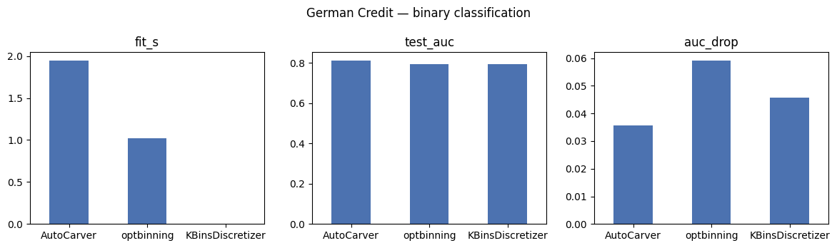
Here, AutoCarver has dropped 6 columns that were not stable on dev set.
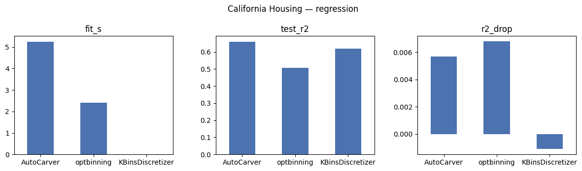
Regression — California Housing
6 numeric demographic features (Latitude / Longitude dropped — see comment in the next cell), 20,640 rows, target = median house value. Same 60 / 20 / 20 split.
[19]:
housing = fetch_california_housing(as_frame=True)
X_reg = housing.frame.drop(columns=['MedHouseVal'])
y_reg = housing.frame['MedHouseVal']

X_train, X_rest, y_train, y_rest = train_test_split(X_reg, y_reg, test_size=0.4, random_state=SEED)
X_dev, X_test, y_dev, y_test = train_test_split(X_rest, y_rest, test_size=0.5, random_state=SEED)

quantitatives = list(X_reg.columns)
categoricals = []

print(f'train={len(X_train)}, dev={len(X_dev)}, test={len(X_test)}')
print(f'quantitatives={len(quantitatives)} ({quantitatives})')
train=12384, dev=4128, test=4128
quantitatives=8 (['MedInc', 'HouseAge', 'AveRooms', 'AveBedrms', 'Population', 'AveOccup', 'Latitude', 'Longitude'])
[20]:
y_train_full = pd.concat([y_train, y_dev])

runs = [(
    'AutoCarver',
    lambda: bin_with_autocarver(X_train, y_train, X_dev, y_dev, X_test, categoricals, quantitatives, 'continuous'),
)]
if HAS_OPTBINNING:
    runs.append((
        'optbinning',
        lambda: bin_with_optbinning(X_train, y_train, X_dev, y_dev, X_test, categoricals, quantitatives, 'continuous'),
    ))
runs.append((
    'KBinsDiscretizer',
    lambda: bin_with_kbins(X_train, X_dev, X_test, categoricals, quantitatives),
))

rows = []
for name, run in runs:
    X_tr, X_te, fit_t, transform_t, carver = run()
    scores = fit_eval_regression(X_tr, X_te, y_train_full, y_test)
    rows.append({
        'library': name,
        'fit_s': round(fit_t, 3),
        'transform_s': round(transform_t, 4),
        'train_r2': round(scores['train_r2'], 4),
        'test_r2': round(scores['test_r2'], 4),
        'r2_drop': round(scores['train_r2'] - scores['test_r2'], 4),
    })

regression_results = pd.DataFrame(rows)
regression_results
------
--- [QuantitativeDiscretizer] Fit Features(['MedInc', 'HouseAge', 'AveRooms', 'AveBedrms', 'Population', 'AveOccup', 'Latitude', 'Longitude'])
 - [ContinuousDiscretizer] Fit Features(['MedInc', 'HouseAge', 'AveRooms', 'AveBedrms', 'Population', 'AveOccup', 'Latitude', 'Longitude'])
 - [OrdinalDiscretizer] Fit Features(['HouseAge', 'Latitude', 'Longitude'])
------

---------
------ [ContinuousCarver] Fit Features(['MedInc', 'HouseAge', 'AveRooms', 'AveBedrms', 'Population', 'AveOccup', 'Latitude', 'Longitude'])
--- [ContinuousCarver] Fit Quantitative('MedInc') (1/8)
 [ContinuousCarver] Raw distribution
| target_mean | frequency | count | |
|---|---|---|---|
| x <= 1.335e+00 | 1.1984 | 0.0250 | 310 |
| 1.335e+00 < x <= 1.593e+00 | 1.0105 | 0.0250 | 310 |
| 1.593e+00 < x <= 1.740e+00 | 1.1133 | 0.0250 | 309 |
| 1.740e+00 < x <= 1.906e+00 | 1.1535 | 0.0252 | 312 |
| 1.906e+00 < x <= 2.029e+00 | 1.2090 | 0.0248 | 307 |
| 2.029e+00 < x <= 2.152e+00 | 1.2141 | 0.0251 | 311 |
| 2.152e+00 < x <= 2.243e+00 | 1.2417 | 0.0250 | 310 |
| 2.243e+00 < x <= 2.350e+00 | 1.3827 | 0.0249 | 308 |
| 2.350e+00 < x <= 2.468e+00 | 1.3614 | 0.0250 | 310 |
| 2.468e+00 < x <= 2.569e+00 | 1.4190 | 0.0250 | 309 |
| 2.569e+00 < x <= 2.655e+00 | 1.5264 | 0.0250 | 310 |
| 2.655e+00 < x <= 2.737e+00 | 1.5428 | 0.0250 | 309 |
| 2.737e+00 < x <= 2.862e+00 | 1.5708 | 0.0250 | 310 |
| 2.862e+00 < x <= 2.974e+00 | 1.6630 | 0.0250 | 310 |
| 2.974e+00 < x <= 3.054e+00 | 1.6270 | 0.0250 | 309 |
| 3.054e+00 < x <= 3.135e+00 | 1.7079 | 0.0250 | 310 |
| 3.135e+00 < x <= 3.216e+00 | 1.8554 | 0.0250 | 309 |
| 3.216e+00 < x <= 3.315e+00 | 1.8373 | 0.0250 | 310 |
| 3.315e+00 < x <= 3.423e+00 | 1.9121 | 0.0250 | 309 |
| 3.423e+00 < x <= 3.531e+00 | 1.9162 | 0.0251 | 311 |
| 3.531e+00 < x <= 3.633e+00 | 1.9678 | 0.0250 | 309 |
| 3.633e+00 < x <= 3.723e+00 | 2.0226 | 0.0250 | 309 |
| 3.723e+00 < x <= 3.839e+00 | 1.9891 | 0.0251 | 311 |
| 3.839e+00 < x <= 3.971e+00 | 2.0493 | 0.0249 | 308 |
| 3.971e+00 < x <= 4.073e+00 | 2.0538 | 0.0252 | 312 |
| 4.073e+00 < x <= 4.179e+00 | 2.2004 | 0.0249 | 308 |
| 4.179e+00 < x <= 4.315e+00 | 2.2417 | 0.0250 | 309 |
| 4.315e+00 < x <= 4.464e+00 | 2.2394 | 0.0250 | 310 |
| 4.464e+00 < x <= 4.611e+00 | 2.2577 | 0.0252 | 312 |
| 4.611e+00 < x <= 4.757e+00 | 2.4351 | 0.0248 | 307 |
| 4.757e+00 < x <= 4.946e+00 | 2.3482 | 0.0250 | 309 |
| 4.946e+00 < x <= 5.117e+00 | 2.4592 | 0.0250 | 310 |
| 5.117e+00 < x <= 5.308e+00 | 2.5784 | 0.0250 | 309 |
| 5.308e+00 < x <= 5.538e+00 | 2.6892 | 0.0250 | 310 |
| 5.538e+00 < x <= 5.828e+00 | 2.7867 | 0.0251 | 311 |
| 5.828e+00 < x <= 6.148e+00 | 3.0943 | 0.0249 | 308 |
| 6.148e+00 < x <= 6.599e+00 | 3.3031 | 0.0250 | 310 |
| 6.599e+00 < x <= 7.313e+00 | 3.6064 | 0.0250 | 309 |
| 7.313e+00 < x <= 8.433e+00 | 4.0191 | 0.0250 | 310 |
| 8.433e+00 < x | 4.7343 | 0.0250 | 310 |
| target_mean | frequency | count |
|---|---|---|
| 1.2507 | 0.0247 | 102 |
| 1.0319 | 0.0262 | 108 |
| 1.1587 | 0.0257 | 106 |
| 1.0855 | 0.0252 | 104 |
| 1.2523 | 0.0225 | 93 |
| 1.2606 | 0.0293 | 121 |
| 1.2643 | 0.0208 | 86 |
| 1.3335 | 0.0274 | 113 |
| 1.4528 | 0.0257 | 106 |
| 1.4887 | 0.0305 | 126 |
| 1.5142 | 0.0237 | 98 |
| 1.6485 | 0.0208 | 86 |
| 1.5544 | 0.0293 | 121 |
| 1.6189 | 0.0257 | 106 |
| 1.7433 | 0.0233 | 96 |
| 1.6369 | 0.0213 | 88 |
| 1.7802 | 0.0276 | 114 |
| 1.9721 | 0.0283 | 117 |
| 1.8287 | 0.0279 | 115 |
| 1.8295 | 0.0242 | 100 |
| 1.9907 | 0.0300 | 124 |
| 1.9517 | 0.0216 | 89 |
| 2.0220 | 0.0269 | 111 |
| 2.1509 | 0.0269 | 111 |
| 2.0977 | 0.0291 | 120 |
| 2.2054 | 0.0225 | 93 |
| 2.2979 | 0.0274 | 113 |
| 2.3553 | 0.0274 | 113 |
| 2.2924 | 0.0184 | 76 |
| 2.4401 | 0.0213 | 88 |
| 2.2931 | 0.0250 | 103 |
| 2.4940 | 0.0237 | 98 |
| 2.6133 | 0.0250 | 103 |
| 2.7177 | 0.0189 | 78 |
| 2.9110 | 0.0276 | 114 |
| 3.0729 | 0.0213 | 88 |
| 3.0759 | 0.0271 | 112 |
| 3.5985 | 0.0228 | 94 |
| 4.0385 | 0.0206 | 85 |
| 4.6131 | 0.0264 | 109 |
[ContinuousCarver] Carved distribution
| target_mean | frequency | count | |
|---|---|---|---|
| x <= 2.47e+00 | 1.2093 | 0.2250 | 2787 |
| 2.47e+00 < x <= 3.13e+00 | 1.5796 | 0.1750 | 2167 |
| 3.13e+00 < x <= 4.07e+00 | 1.9560 | 0.2251 | 2788 |
| 4.07e+00 < x <= 5.83e+00 | 2.4238 | 0.2499 | 3095 |
| 5.83e+00 < x | 3.7524 | 0.1249 | 1547 |
| target_mean | frequency | count |
|---|---|---|
| 1.2323 | 0.2275 | 939 |
| 1.5934 | 0.1747 | 721 |
| 1.9604 | 0.2425 | 1001 |
| 2.4652 | 0.2372 | 979 |
| 3.6870 | 0.1182 | 488 |
--- [ContinuousCarver] Fit Quantitative('HouseAge') (2/8)
 [ContinuousCarver] Raw distribution
| target_mean | frequency | count | |
|---|---|---|---|
| x <= 5.00e+00 | 2.2358 | 0.0271 | 336 |
| 5.00e+00 < x <= 8.00e+00 | 1.9727 | 0.0263 | 326 |
| 8.00e+00 < x <= 1.10e+01 | 1.8133 | 0.0352 | 436 |
| 1.10e+01 < x <= 1.40e+01 | 1.8538 | 0.0468 | 579 |
| 1.40e+01 < x <= 1.60e+01 | 1.9355 | 0.0652 | 807 |
| 1.60e+01 < x <= 1.70e+01 | 1.8929 | 0.0319 | 395 |
| 1.70e+01 < x <= 1.80e+01 | 1.9455 | 0.0276 | 342 |
| 1.80e+01 < x <= 2.00e+01 | 1.9470 | 0.0470 | 582 |
| 2.00e+01 < x <= 2.30e+01 | 1.9934 | 0.0632 | 783 |
| 2.30e+01 < x <= 2.50e+01 | 2.1713 | 0.0480 | 595 |
| 2.50e+01 < x <= 2.60e+01 | 2.0937 | 0.0304 | 377 |
| 2.60e+01 < x <= 2.70e+01 | 2.0568 | 0.0245 | 303 |
| 2.70e+01 < x <= 2.80e+01 | 1.9827 | 0.0241 | 299 |
| 2.80e+01 < x <= 2.90e+01 | 2.0203 | 0.0232 | 287 |
| 2.90e+01 < x <= 3.00e+01 | 2.0515 | 0.0236 | 292 |
| 3.00e+01 < x <= 3.20e+01 | 2.0453 | 0.0484 | 599 |
| 3.20e+01 < x <= 3.30e+01 | 2.0343 | 0.0316 | 391 |
| 3.30e+01 < x <= 3.40e+01 | 2.1357 | 0.0320 | 396 |
| 3.40e+01 < x <= 3.50e+01 | 2.0004 | 0.0399 | 494 |
| 3.50e+01 < x <= 3.60e+01 | 2.1148 | 0.0437 | 541 |
| 3.60e+01 < x <= 3.70e+01 | 2.0004 | 0.0257 | 318 |
| 3.70e+01 < x <= 3.90e+01 | 2.0133 | 0.0355 | 440 |
| 3.90e+01 < x <= 4.20e+01 | 2.0148 | 0.0440 | 545 |
| 4.20e+01 < x <= 4.40e+01 | 2.0742 | 0.0351 | 435 |
| 4.40e+01 < x <= 4.70e+01 | 2.0852 | 0.0343 | 425 |
| 4.70e+01 < x | 2.5848 | 0.0857 | 1061 |
| target_mean | frequency | count |
|---|---|---|
| 2.0720 | 0.0245 | 101 |
| 1.9201 | 0.0269 | 111 |
| 1.9054 | 0.0344 | 142 |
| 1.8581 | 0.0412 | 170 |
| 1.8826 | 0.0606 | 250 |
| 1.8592 | 0.0375 | 155 |
| 1.8799 | 0.0283 | 117 |
| 1.8746 | 0.0436 | 180 |
| 2.1128 | 0.0577 | 238 |
| 2.0847 | 0.0579 | 239 |
| 2.0778 | 0.0296 | 122 |
| 2.1784 | 0.0216 | 89 |
| 2.2242 | 0.0208 | 86 |
| 1.7802 | 0.0213 | 88 |
| 1.7629 | 0.0233 | 96 |
| 2.0493 | 0.0504 | 208 |
| 1.9343 | 0.0259 | 107 |
| 2.0837 | 0.0349 | 144 |
| 2.1957 | 0.0417 | 172 |
| 2.0157 | 0.0431 | 178 |
| 2.2006 | 0.0296 | 122 |
| 2.0026 | 0.0351 | 145 |
| 1.9358 | 0.0499 | 206 |
| 2.0117 | 0.0312 | 129 |
| 2.0839 | 0.0380 | 157 |
| 2.5968 | 0.0911 | 376 |
[ContinuousCarver] Carved distribution
| target_mean | frequency | count | |
|---|---|---|---|
| x <= 2.30e+01 | 1.9466 | 0.3703 | 4586 |
| 2.30e+01 < x <= 2.60e+01 | 2.1412 | 0.0785 | 972 |
| 2.60e+01 < x <= 3.60e+01 | 2.0526 | 0.2909 | 3602 |
| 3.60e+01 < x <= 4.70e+01 | 2.0381 | 0.1747 | 2163 |
| 4.70e+01 < x | 2.5848 | 0.0857 | 1061 |
| target_mean | frequency | count |
|---|---|---|
| 1.9316 | 0.3547 | 1464 |
| 2.0824 | 0.0875 | 361 |
| 2.0383 | 0.2829 | 1168 |
| 2.0347 | 0.1839 | 759 |
| 2.5968 | 0.0911 | 376 |
--- [ContinuousCarver] Fit Quantitative('AveRooms') (3/8)
 [ContinuousCarver] Raw distribution
| target_mean | frequency | count | |
|---|---|---|---|
| x <= 3.066e+00 | 1.9506 | 0.0250 | 310 |
| 3.066e+00 < x <= 3.432e+00 | 1.8880 | 0.0250 | 310 |
| 3.432e+00 < x <= 3.647e+00 | 1.8233 | 0.0250 | 309 |
| 3.647e+00 < x <= 3.792e+00 | 1.8292 | 0.0250 | 310 |
| 3.792e+00 < x <= 3.933e+00 | 1.7847 | 0.0250 | 309 |
| 3.933e+00 < x <= 4.052e+00 | 1.8499 | 0.0250 | 310 |
| 4.052e+00 < x <= 4.168e+00 | 1.8718 | 0.0250 | 310 |
| 4.168e+00 < x <= 4.276e+00 | 1.8333 | 0.0250 | 309 |
| 4.276e+00 < x <= 4.365e+00 | 1.7965 | 0.0250 | 310 |
| 4.365e+00 < x <= 4.454e+00 | 1.6952 | 0.0250 | 309 |
| 4.454e+00 < x <= 4.536e+00 | 1.7535 | 0.0250 | 310 |
| 4.536e+00 < x <= 4.621e+00 | 1.7952 | 0.0250 | 309 |
| 4.621e+00 < x <= 4.705e+00 | 1.8465 | 0.0250 | 310 |
| 4.705e+00 < x <= 4.794e+00 | 1.7486 | 0.0250 | 310 |
| 4.794e+00 < x <= 4.874e+00 | 1.7719 | 0.0250 | 309 |
| 4.874e+00 < x <= 4.941e+00 | 1.7219 | 0.0251 | 311 |
| 4.941e+00 < x <= 5.014e+00 | 1.7176 | 0.0249 | 308 |
| 5.014e+00 < x <= 5.088e+00 | 1.7707 | 0.0250 | 310 |
| 5.088e+00 < x <= 5.160e+00 | 1.7918 | 0.0250 | 309 |
| 5.160e+00 < x <= 5.233e+00 | 1.7791 | 0.0250 | 310 |
| 5.233e+00 < x <= 5.315e+00 | 1.8209 | 0.0250 | 310 |
| 5.315e+00 < x <= 5.384e+00 | 1.9107 | 0.0250 | 309 |
| 5.384e+00 < x <= 5.460e+00 | 1.7728 | 0.0250 | 310 |
| 5.460e+00 < x <= 5.532e+00 | 1.8996 | 0.0250 | 309 |
| 5.532e+00 < x <= 5.616e+00 | 1.8872 | 0.0250 | 310 |
| 5.616e+00 < x <= 5.694e+00 | 1.9905 | 0.0250 | 309 |
| 5.694e+00 < x <= 5.778e+00 | 2.0029 | 0.0250 | 310 |
| 5.778e+00 < x <= 5.858e+00 | 2.0107 | 0.0250 | 310 |
| 5.858e+00 < x <= 5.959e+00 | 2.1137 | 0.0250 | 309 |
| 5.959e+00 < x <= 6.059e+00 | 2.0469 | 0.0250 | 310 |
| 6.059e+00 < x <= 6.157e+00 | 2.1450 | 0.0250 | 309 |
| 6.157e+00 < x <= 6.270e+00 | 2.2477 | 0.0250 | 310 |
| 6.270e+00 < x <= 6.396e+00 | 2.3495 | 0.0250 | 309 |
| 6.396e+00 < x <= 6.543e+00 | 2.4232 | 0.0250 | 310 |
| 6.543e+00 < x <= 6.717e+00 | 2.6241 | 0.0250 | 310 |
| 6.717e+00 < x <= 6.946e+00 | 2.7573 | 0.0250 | 309 |
| 6.946e+00 < x <= 7.233e+00 | 3.0763 | 0.0250 | 310 |
| 7.233e+00 < x <= 7.637e+00 | 3.1118 | 0.0250 | 309 |
| 7.637e+00 < x <= 8.324e+00 | 3.5846 | 0.0250 | 310 |
| 8.324e+00 < x | 2.7391 | 0.0250 | 310 |
| target_mean | frequency | count |
|---|---|---|
| 2.0908 | 0.0233 | 96 |
| 1.8579 | 0.0264 | 109 |
| 2.0031 | 0.0242 | 100 |
| 1.8060 | 0.0274 | 113 |
| 1.8137 | 0.0240 | 99 |
| 1.7725 | 0.0211 | 87 |
| 1.7723 | 0.0283 | 117 |
| 1.7839 | 0.0247 | 102 |
| 1.7902 | 0.0286 | 118 |
| 1.8121 | 0.0264 | 109 |
| 1.6265 | 0.0264 | 109 |
| 1.8349 | 0.0276 | 114 |
| 1.8339 | 0.0247 | 102 |
| 1.7725 | 0.0342 | 141 |
| 1.8188 | 0.0254 | 105 |
| 1.8480 | 0.0191 | 79 |
| 1.8333 | 0.0235 | 97 |
| 1.8191 | 0.0266 | 110 |
| 1.7419 | 0.0266 | 110 |
| 1.7642 | 0.0220 | 91 |
| 1.7645 | 0.0303 | 125 |
| 1.7917 | 0.0266 | 110 |
| 1.8651 | 0.0262 | 108 |
| 1.8645 | 0.0274 | 113 |
| 1.8082 | 0.0286 | 118 |
| 1.8483 | 0.0177 | 73 |
| 2.0778 | 0.0240 | 99 |
| 2.0005 | 0.0187 | 77 |
| 1.9724 | 0.0291 | 120 |
| 2.2623 | 0.0235 | 97 |
| 2.0818 | 0.0230 | 95 |
| 2.2889 | 0.0250 | 103 |
| 2.3280 | 0.0213 | 88 |
| 2.5373 | 0.0254 | 105 |
| 2.6787 | 0.0201 | 83 |
| 2.7457 | 0.0211 | 87 |
| 3.0108 | 0.0303 | 125 |
| 3.1596 | 0.0233 | 96 |
| 3.4340 | 0.0235 | 97 |
| 2.7568 | 0.0245 | 101 |
[ContinuousCarver] Carved distribution
| target_mean | frequency | count | |
|---|---|---|---|
| x <= 3.43e+00 | 1.9193 | 0.0501 | 620 |
| 3.43e+00 < x <= 5.62e+00 | 1.8031 | 0.5749 | 7120 |
| 5.62e+00 < x <= 6.16e+00 | 2.0516 | 0.1500 | 1857 |
| 6.16e+00 < x <= 6.54e+00 | 2.3401 | 0.0750 | 929 |
| 6.54e+00 < x | 2.9823 | 0.1500 | 1858 |
| target_mean | frequency | count |
|---|---|---|
| 1.9670 | 0.0497 | 205 |
| 1.8045 | 0.6000 | 2477 |
| 2.0474 | 0.1359 | 561 |
| 2.3886 | 0.0717 | 296 |
| 2.9752 | 0.1427 | 589 |
--- [ContinuousCarver] Fit Quantitative('AveBedrms') (4/8)
 [ContinuousCarver] Raw distribution
| target_mean | frequency | count | |
|---|---|---|---|
| x <= 9.1220e-01 | 2.0511 | 0.0250 | 310 |
| 9.1220e-01 < x <= 9.4022e-01 | 2.1264 | 0.0250 | 310 |
| 9.4022e-01 < x <= 9.5595e-01 | 2.0638 | 0.0250 | 309 |
| 9.5595e-01 < x <= 9.6743e-01 | 2.0756 | 0.0251 | 311 |
| 9.6743e-01 < x <= 9.7590e-01 | 2.2562 | 0.0249 | 308 |
| 9.7590e-01 < x <= 9.8343e-01 | 2.1709 | 0.0250 | 310 |
| 9.8343e-01 < x <= 9.8987e-01 | 2.1450 | 0.0250 | 310 |
| 9.8987e-01 < x <= 9.9592e-01 | 2.1772 | 0.0250 | 309 |
| 9.9592e-01 < x <= 1.0019e+00 | 2.1915 | 0.0251 | 311 |
| 1.0019e+00 < x <= 1.0068e+00 | 2.0949 | 0.0249 | 308 |
| 1.0068e+00 < x <= 1.0112e+00 | 2.2440 | 0.0250 | 310 |
| 1.0112e+00 < x <= 1.0156e+00 | 2.1687 | 0.0250 | 310 |
| 1.0156e+00 < x <= 1.0204e+00 | 2.1723 | 0.0250 | 309 |
| 1.0204e+00 < x <= 1.0250e+00 | 2.2003 | 0.0254 | 314 |
| 1.0250e+00 < x <= 1.0290e+00 | 2.1324 | 0.0246 | 305 |
| 1.0290e+00 < x <= 1.0331e+00 | 2.1840 | 0.0250 | 310 |
| 1.0331e+00 < x <= 1.0369e+00 | 2.0321 | 0.0250 | 309 |
| 1.0369e+00 < x <= 1.0412e+00 | 2.1746 | 0.0250 | 310 |
| 1.0412e+00 < x <= 1.0453e+00 | 2.2536 | 0.0250 | 309 |
| 1.0453e+00 < x <= 1.0493e+00 | 2.1546 | 0.0250 | 310 |
| 1.0493e+00 < x <= 1.0534e+00 | 2.0738 | 0.0251 | 311 |
| 1.0534e+00 < x <= 1.0574e+00 | 2.1224 | 0.0249 | 308 |
| 1.0574e+00 < x <= 1.0615e+00 | 2.0414 | 0.0250 | 310 |
| 1.0615e+00 < x <= 1.0662e+00 | 2.1569 | 0.0251 | 311 |
| 1.0662e+00 < x <= 1.0712e+00 | 2.0972 | 0.0250 | 309 |
| 1.0712e+00 < x <= 1.0763e+00 | 2.0714 | 0.0249 | 308 |
| 1.0763e+00 < x <= 1.0816e+00 | 2.0244 | 0.0250 | 310 |
| 1.0816e+00 < x <= 1.0874e+00 | 2.0135 | 0.0252 | 312 |
| 1.0874e+00 < x <= 1.0933e+00 | 2.2239 | 0.0249 | 308 |
| 1.0933e+00 < x <= 1.1000e+00 | 2.0244 | 0.0262 | 324 |
| 1.1000e+00 < x <= 1.1071e+00 | 2.0077 | 0.0242 | 300 |
| 1.1071e+00 < x <= 1.1160e+00 | 1.9564 | 0.0245 | 304 |
| 1.1160e+00 < x <= 1.1267e+00 | 2.0077 | 0.0250 | 310 |
| 1.1267e+00 < x <= 1.1387e+00 | 1.9305 | 0.0250 | 309 |
| 1.1387e+00 < x <= 1.1538e+00 | 1.8130 | 0.0258 | 319 |
| 1.1538e+00 < x <= 1.1739e+00 | 1.8060 | 0.0242 | 300 |
| 1.1739e+00 < x <= 1.2074e+00 | 1.9109 | 0.0250 | 310 |
| 1.2074e+00 < x <= 1.2730e+00 | 1.8950 | 0.0250 | 309 |
| 1.2730e+00 < x <= 1.5018e+00 | 1.7962 | 0.0250 | 310 |
| 1.5018e+00 < x | 1.4931 | 0.0250 | 310 |
| target_mean | frequency | count |
|---|---|---|
| 1.7961 | 0.0252 | 104 |
| 2.0098 | 0.0298 | 123 |
| 2.3039 | 0.0257 | 106 |
| 2.2390 | 0.0262 | 108 |
| 2.3293 | 0.0240 | 99 |
| 1.9318 | 0.0194 | 80 |
| 2.1575 | 0.0199 | 82 |
| 2.1740 | 0.0291 | 120 |
| 2.2207 | 0.0337 | 139 |
| 2.1811 | 0.0233 | 96 |
| 2.0475 | 0.0262 | 108 |
| 2.2743 | 0.0218 | 90 |
| 2.2627 | 0.0293 | 121 |
| 2.1068 | 0.0247 | 102 |
| 2.4459 | 0.0228 | 94 |
| 2.1280 | 0.0269 | 111 |
| 2.1193 | 0.0240 | 99 |
| 2.2280 | 0.0259 | 107 |
| 2.0336 | 0.0237 | 98 |
| 2.0195 | 0.0216 | 89 |
| 1.9898 | 0.0235 | 97 |
| 2.2270 | 0.0216 | 89 |
| 1.9244 | 0.0254 | 105 |
| 2.1509 | 0.0237 | 98 |
| 2.2223 | 0.0274 | 113 |
| 1.9654 | 0.0271 | 112 |
| 2.1085 | 0.0257 | 106 |
| 2.0332 | 0.0240 | 99 |
| 1.9262 | 0.0264 | 109 |
| 2.1139 | 0.0274 | 113 |
| 1.9025 | 0.0225 | 93 |
| 1.8628 | 0.0271 | 112 |
| 1.9501 | 0.0259 | 107 |
| 2.0231 | 0.0206 | 85 |
| 1.8622 | 0.0271 | 112 |
| 1.8137 | 0.0250 | 103 |
| 2.0399 | 0.0259 | 107 |
| 1.6392 | 0.0218 | 90 |
| 1.7221 | 0.0250 | 103 |
| 1.6019 | 0.0240 | 99 |
[ContinuousCarver] Carved distribution
| target_mean | frequency | count | |
|---|---|---|---|
| x <= 1.049e+00 | 2.1535 | 0.5000 | 6192 |
| 1.049e+00 < x <= 1.093e+00 | 2.0915 | 0.2250 | 2787 |
| 1.093e+00 < x <= 1.139e+00 | 1.9857 | 0.1249 | 1547 |
| 1.139e+00 < x <= 1.273e+00 | 1.8563 | 0.1000 | 1238 |
| 1.273e+00 < x | 1.6446 | 0.0501 | 620 |
| target_mean | frequency | count |
|---|---|---|
| 2.1526 | 0.5029 | 2076 |
| 2.0582 | 0.2248 | 928 |
| 1.9707 | 0.1235 | 510 |
| 1.8475 | 0.0998 | 412 |
| 1.6632 | 0.0489 | 202 |
--- [ContinuousCarver] Fit Quantitative('Population') (5/8)
 [ContinuousCarver] Raw distribution
| target_mean | frequency | count | |
|---|---|---|---|
| x <= 2.08e+02 | 1.9050 | 0.0251 | 311 |
| 2.08e+02 < x <= 3.53e+02 | 2.0277 | 0.0251 | 311 |
| 3.53e+02 < x <= 4.42e+02 | 2.0655 | 0.0250 | 310 |
| 4.42e+02 < x <= 5.12e+02 | 2.2067 | 0.0249 | 308 |
| 5.12e+02 < x <= 5.75e+02 | 2.1327 | 0.0250 | 310 |
| 5.75e+02 < x <= 6.27e+02 | 2.0731 | 0.0250 | 310 |
| 6.27e+02 < x <= 6.75e+02 | 2.3627 | 0.0249 | 308 |
| 6.75e+02 < x <= 7.16e+02 | 2.2006 | 0.0250 | 309 |
| 7.16e+02 < x <= 7.56e+02 | 2.0900 | 0.0253 | 313 |
| 7.56e+02 < x <= 7.94e+02 | 2.0191 | 0.0251 | 311 |
| 7.94e+02 < x <= 8.32e+02 | 2.3248 | 0.0251 | 311 |
| 8.32e+02 < x <= 8.67e+02 | 2.0763 | 0.0253 | 313 |
| 8.67e+02 < x <= 9.02e+02 | 2.0313 | 0.0247 | 306 |
| 9.02e+02 < x <= 9.40e+02 | 2.1185 | 0.0247 | 306 |
| 9.40e+02 < x <= 9.78e+02 | 2.1790 | 0.0253 | 313 |
| 9.78e+02 < x <= 1.02e+03 | 2.0746 | 0.0249 | 308 |
| 1.02e+03 < x <= 1.06e+03 | 1.9522 | 0.0247 | 306 |
| 1.06e+03 < x <= 1.09e+03 | 2.1186 | 0.0250 | 310 |
| 1.09e+03 < x <= 1.13e+03 | 2.0592 | 0.0252 | 312 |
| 1.13e+03 < x <= 1.17e+03 | 2.0640 | 0.0252 | 312 |
| 1.17e+03 < x <= 1.22e+03 | 2.0134 | 0.0249 | 308 |
| 1.22e+03 < x <= 1.26e+03 | 2.1690 | 0.0250 | 310 |
| 1.26e+03 < x <= 1.30e+03 | 2.0558 | 0.0248 | 307 |
| 1.30e+03 < x <= 1.35e+03 | 1.9711 | 0.0249 | 308 |
| 1.35e+03 < x <= 1.41e+03 | 2.0185 | 0.0250 | 310 |
| 1.41e+03 < x <= 1.46e+03 | 2.0004 | 0.0251 | 311 |
| 1.46e+03 < x <= 1.52e+03 | 2.0911 | 0.0248 | 307 |
| 1.52e+03 < x <= 1.59e+03 | 2.1322 | 0.0254 | 315 |
| 1.59e+03 < x <= 1.66e+03 | 1.9949 | 0.0246 | 305 |
| 1.66e+03 < x <= 1.73e+03 | 2.0233 | 0.0250 | 309 |
| 1.73e+03 < x <= 1.82e+03 | 1.8946 | 0.0253 | 313 |
| 1.82e+03 < x <= 1.91e+03 | 1.9504 | 0.0247 | 306 |
| 1.91e+03 < x <= 2.02e+03 | 2.0074 | 0.0250 | 310 |
| 2.02e+03 < x <= 2.16e+03 | 2.0213 | 0.0250 | 310 |
| 2.16e+03 < x <= 2.32e+03 | 2.0541 | 0.0250 | 309 |
| 2.32e+03 < x <= 2.56e+03 | 2.0757 | 0.0250 | 310 |
| 2.56e+03 < x <= 2.86e+03 | 2.0142 | 0.0250 | 309 |
| 2.86e+03 < x <= 3.28e+03 | 1.9196 | 0.0250 | 309 |
| 3.28e+03 < x <= 4.25e+03 | 2.0439 | 0.0250 | 310 |
| 4.25e+03 < x | 2.0010 | 0.0250 | 310 |
| target_mean | frequency | count |
|---|---|---|
| 1.9895 | 0.0269 | 111 |
| 1.8189 | 0.0271 | 112 |
| 2.1479 | 0.0271 | 112 |
| 2.2434 | 0.0266 | 110 |
| 2.1281 | 0.0269 | 111 |
| 2.2908 | 0.0257 | 106 |
| 2.0926 | 0.0283 | 117 |
| 2.1757 | 0.0213 | 88 |
| 2.2182 | 0.0259 | 107 |
| 2.1433 | 0.0286 | 118 |
| 2.0769 | 0.0293 | 121 |
| 2.1889 | 0.0240 | 99 |
| 2.0488 | 0.0218 | 90 |
| 2.1585 | 0.0247 | 102 |
| 2.0699 | 0.0259 | 107 |
| 2.0396 | 0.0247 | 102 |
| 1.9843 | 0.0254 | 105 |
| 2.1062 | 0.0213 | 88 |
| 1.9823 | 0.0242 | 100 |
| 2.1353 | 0.0271 | 112 |
| 2.1132 | 0.0230 | 95 |
| 1.9696 | 0.0252 | 104 |
| 2.1243 | 0.0196 | 81 |
| 1.9774 | 0.0245 | 101 |
| 1.8002 | 0.0245 | 101 |
| 2.1500 | 0.0264 | 109 |
| 1.9471 | 0.0293 | 121 |
| 1.9535 | 0.0262 | 108 |
| 2.0915 | 0.0274 | 113 |
| 2.0390 | 0.0228 | 94 |
| 2.1380 | 0.0211 | 87 |
| 1.9706 | 0.0203 | 84 |
| 1.8717 | 0.0264 | 109 |
| 1.9082 | 0.0247 | 102 |
| 2.0895 | 0.0233 | 96 |
| 1.8131 | 0.0266 | 110 |
| 2.0019 | 0.0269 | 111 |
| 2.0234 | 0.0201 | 83 |
| 2.1558 | 0.0262 | 108 |
| 2.0339 | 0.0225 | 93 |
[ContinuousCarver] Carved distribution
| target_mean | frequency | count | |
|---|---|---|---|
| x <= 3.53e+02 | 1.9663 | 0.0502 | 622 |
| 3.53e+02 < x <= 8.32e+02 | 2.1636 | 0.2253 | 2790 |
| 8.32e+02 < x <= 1.73e+03 | 2.0604 | 0.4745 | 5876 |
| 1.73e+03 < x <= 2.16e+03 | 1.9683 | 0.1000 | 1239 |
| 2.16e+03 < x | 2.0181 | 0.1500 | 1857 |
| target_mean | frequency | count |
|---|---|---|
| 1.9038 | 0.0540 | 223 |
| 2.1659 | 0.2398 | 990 |
| 2.0445 | 0.4680 | 1932 |
| 1.9639 | 0.0925 | 382 |
| 2.0169 | 0.1456 | 601 |
--- [ContinuousCarver] Fit Quantitative('AveOccup') (6/8)
 [ContinuousCarver] Raw distribution
| target_mean | frequency | count | |
|---|---|---|---|
| x <= 1.699e+00 | 2.6141 | 0.0250 | 310 |
| 1.699e+00 < x <= 1.868e+00 | 2.7986 | 0.0250 | 310 |
| 1.868e+00 < x <= 1.976e+00 | 2.6979 | 0.0250 | 309 |
| 1.976e+00 < x <= 2.071e+00 | 2.5558 | 0.0250 | 310 |
| 2.071e+00 < x <= 2.161e+00 | 2.4582 | 0.0250 | 309 |
| 2.161e+00 < x <= 2.228e+00 | 2.2757 | 0.0250 | 310 |
| 2.228e+00 < x <= 2.288e+00 | 2.3592 | 0.0250 | 310 |
| 2.288e+00 < x <= 2.341e+00 | 2.2507 | 0.0250 | 309 |
| 2.341e+00 < x <= 2.388e+00 | 2.1371 | 0.0250 | 310 |
| 2.388e+00 < x <= 2.435e+00 | 2.2708 | 0.0250 | 309 |
| 2.435e+00 < x <= 2.475e+00 | 2.1989 | 0.0250 | 310 |
| 2.475e+00 < x <= 2.515e+00 | 2.1564 | 0.0250 | 309 |
| 2.515e+00 < x <= 2.557e+00 | 2.1279 | 0.0250 | 310 |
| 2.557e+00 < x <= 2.598e+00 | 2.2428 | 0.0250 | 310 |
| 2.598e+00 < x <= 2.639e+00 | 2.1116 | 0.0250 | 309 |
| 2.639e+00 < x <= 2.674e+00 | 2.2343 | 0.0250 | 310 |
| 2.674e+00 < x <= 2.712e+00 | 2.0489 | 0.0250 | 309 |
| 2.712e+00 < x <= 2.746e+00 | 2.2196 | 0.0250 | 310 |
| 2.746e+00 < x <= 2.784e+00 | 2.1211 | 0.0250 | 309 |
| 2.784e+00 < x <= 2.824e+00 | 2.2645 | 0.0250 | 310 |
| 2.824e+00 < x <= 2.861e+00 | 2.1565 | 0.0251 | 311 |
| 2.861e+00 < x <= 2.899e+00 | 2.2323 | 0.0250 | 309 |
| 2.899e+00 < x <= 2.943e+00 | 2.0714 | 0.0250 | 309 |
| 2.943e+00 < x <= 2.984e+00 | 2.0495 | 0.0250 | 309 |
| 2.984e+00 < x <= 3.026e+00 | 1.9917 | 0.0250 | 310 |
| 3.026e+00 < x <= 3.071e+00 | 1.9623 | 0.0250 | 309 |
| 3.071e+00 < x <= 3.117e+00 | 2.0491 | 0.0250 | 310 |
| 3.117e+00 < x <= 3.168e+00 | 1.9336 | 0.0250 | 310 |
| 3.168e+00 < x <= 3.221e+00 | 1.9472 | 0.0250 | 310 |
| 3.221e+00 < x <= 3.279e+00 | 1.8938 | 0.0250 | 309 |
| 3.279e+00 < x <= 3.344e+00 | 1.8804 | 0.0250 | 309 |
| 3.344e+00 < x <= 3.424e+00 | 1.8724 | 0.0250 | 310 |
| 3.424e+00 < x <= 3.508e+00 | 1.8000 | 0.0250 | 309 |
| 3.508e+00 < x <= 3.606e+00 | 1.6571 | 0.0250 | 310 |
| 3.606e+00 < x <= 3.719e+00 | 1.5624 | 0.0250 | 310 |
| 3.719e+00 < x <= 3.870e+00 | 1.5709 | 0.0250 | 309 |
| 3.870e+00 < x <= 4.089e+00 | 1.4854 | 0.0250 | 310 |
| 4.089e+00 < x <= 4.317e+00 | 1.4240 | 0.0250 | 309 |
| 4.317e+00 < x <= 4.705e+00 | 1.3233 | 0.0250 | 310 |
| 4.705e+00 < x | 1.5280 | 0.0250 | 310 |
| target_mean | frequency | count |
|---|---|---|
| 2.7524 | 0.0220 | 91 |
| 2.7763 | 0.0293 | 121 |
| 2.6502 | 0.0257 | 106 |
| 2.5990 | 0.0242 | 100 |
| 2.4828 | 0.0296 | 122 |
| 2.4039 | 0.0247 | 102 |
| 2.2567 | 0.0281 | 116 |
| 2.4137 | 0.0230 | 95 |
| 2.3471 | 0.0211 | 87 |
| 2.2425 | 0.0300 | 124 |
| 2.0911 | 0.0252 | 104 |
| 2.2072 | 0.0259 | 107 |
| 2.1370 | 0.0262 | 108 |
| 2.0973 | 0.0281 | 116 |
| 2.0188 | 0.0230 | 95 |
| 2.0825 | 0.0225 | 93 |
| 2.2615 | 0.0247 | 102 |
| 2.0114 | 0.0213 | 88 |
| 2.2314 | 0.0257 | 106 |
| 2.0203 | 0.0233 | 96 |
| 2.0908 | 0.0286 | 118 |
| 1.8887 | 0.0233 | 96 |
| 1.9894 | 0.0250 | 103 |
| 2.2316 | 0.0228 | 94 |
| 2.0891 | 0.0291 | 120 |
| 1.9787 | 0.0223 | 92 |
| 2.0818 | 0.0279 | 115 |
| 1.8602 | 0.0203 | 84 |
| 1.9611 | 0.0189 | 78 |
| 1.7265 | 0.0230 | 95 |
| 1.7789 | 0.0259 | 107 |
| 1.8341 | 0.0274 | 113 |
| 1.6481 | 0.0211 | 87 |
| 1.6989 | 0.0247 | 102 |
| 1.6267 | 0.0271 | 112 |
| 1.5547 | 0.0250 | 103 |
| 1.4150 | 0.0293 | 121 |
| 1.5364 | 0.0220 | 91 |
| 1.4245 | 0.0262 | 108 |
| 1.5598 | 0.0266 | 110 |
[ContinuousCarver] Carved distribution
| target_mean | frequency | count | |
|---|---|---|---|
| x <= 2.16e+00 | 2.6250 | 0.1250 | 1548 |
| 2.16e+00 < x <= 2.90e+00 | 2.2005 | 0.4251 | 5264 |
| 2.90e+00 < x <= 3.51e+00 | 1.9501 | 0.2749 | 3404 |
| 3.51e+00 < x <= 3.87e+00 | 1.5968 | 0.0750 | 929 |
| 3.87e+00 < x | 1.4402 | 0.1000 | 1239 |
| target_mean | frequency | count |
|---|---|---|
| 2.6484 | 0.1308 | 540 |
| 2.1665 | 0.4247 | 1753 |
| 1.9311 | 0.2636 | 1088 |
| 1.6265 | 0.0768 | 317 |
| 1.4801 | 0.1042 | 430 |
--- [ContinuousCarver] Fit Quantitative('Latitude') (7/8)
 [ContinuousCarver] Raw distribution
| target_mean | frequency | count | |
|---|---|---|---|
| x <= 3.275e+01 | 1.5912 | 0.0287 | 355 |
| 3.275e+01 < x <= 3.321e+01 | 2.0299 | 0.0466 | 577 |
| 3.321e+01 < x <= 3.365e+01 | 2.7833 | 0.0279 | 345 |
| 3.365e+01 < x <= 3.374e+01 | 2.4326 | 0.0268 | 332 |
| 3.374e+01 < x <= 3.379e+01 | 2.1829 | 0.0262 | 325 |
| 3.379e+01 < x <= 3.383e+01 | 2.4232 | 0.0229 | 283 |
| 3.383e+01 < x <= 3.387e+01 | 2.3003 | 0.0241 | 299 |
| 3.387e+01 < x <= 3.391e+01 | 2.1570 | 0.0279 | 345 |
| 3.391e+01 < x <= 3.394e+01 | 1.6300 | 0.0242 | 300 |
| 3.394e+01 < x <= 3.397e+01 | 1.8594 | 0.0225 | 279 |
| 3.397e+01 < x <= 3.400e+01 | 1.9482 | 0.0224 | 278 |
| 3.400e+01 < x <= 3.403e+01 | 2.1267 | 0.0277 | 343 |
| 3.403e+01 < x <= 3.406e+01 | 2.4021 | 0.0339 | 420 |
| 3.406e+01 < x <= 3.410e+01 | 2.1760 | 0.0417 | 516 |
| 3.410e+01 < x <= 3.413e+01 | 2.3646 | 0.0242 | 300 |
| 3.413e+01 < x <= 3.417e+01 | 2.7771 | 0.0301 | 373 |
| 3.417e+01 < x <= 3.427e+01 | 2.4100 | 0.0435 | 539 |
| 3.427e+01 < x <= 3.453e+01 | 2.4559 | 0.0240 | 297 |
| 3.453e+01 < x <= 3.532e+01 | 1.4914 | 0.0246 | 305 |
| 3.532e+01 < x <= 3.623e+01 | 0.9208 | 0.0250 | 310 |
| 3.623e+01 < x <= 3.672e+01 | 1.2441 | 0.0262 | 324 |
| 3.672e+01 < x <= 3.697e+01 | 1.3129 | 0.0253 | 313 |
| 3.697e+01 < x <= 3.729e+01 | 2.6241 | 0.0239 | 296 |
| 3.729e+01 < x <= 3.737e+01 | 2.6574 | 0.0258 | 320 |
| 3.737e+01 < x <= 3.753e+01 | 3.0105 | 0.0255 | 316 |
| 3.753e+01 < x <= 3.765e+01 | 2.4197 | 0.0243 | 301 |
| 3.765e+01 < x <= 3.772e+01 | 2.1174 | 0.0256 | 317 |
| 3.772e+01 < x <= 3.777e+01 | 2.5537 | 0.0286 | 354 |
| 3.777e+01 < x <= 3.793e+01 | 2.6887 | 0.0459 | 569 |
| 3.793e+01 < x <= 3.800e+01 | 1.7622 | 0.0250 | 310 |
| 3.800e+01 < x <= 3.826e+01 | 1.5924 | 0.0243 | 301 |
| 3.826e+01 < x <= 3.850e+01 | 1.8570 | 0.0254 | 315 |
| 3.850e+01 < x <= 3.863e+01 | 1.3981 | 0.0241 | 298 |
| 3.863e+01 < x <= 3.898e+01 | 1.3962 | 0.0251 | 311 |
| 3.898e+01 < x <= 3.975e+01 | 1.1241 | 0.0255 | 316 |
| 3.975e+01 < x | 0.8442 | 0.0244 | 302 |
| target_mean | frequency | count |
|---|---|---|
| 1.5761 | 0.0320 | 132 |
| 2.0768 | 0.0552 | 228 |
| 2.7115 | 0.0264 | 109 |
| 2.4368 | 0.0262 | 108 |
| 2.2910 | 0.0291 | 120 |
| 2.3528 | 0.0220 | 91 |
| 2.3233 | 0.0233 | 96 |
| 2.0937 | 0.0368 | 152 |
| 1.6319 | 0.0230 | 95 |
| 1.7992 | 0.0235 | 97 |
| 1.9408 | 0.0250 | 103 |
| 2.1292 | 0.0250 | 103 |
| 2.3261 | 0.0334 | 138 |
| 2.2762 | 0.0443 | 183 |
| 2.2228 | 0.0216 | 89 |
| 2.8224 | 0.0303 | 125 |
| 2.2938 | 0.0465 | 192 |
| 2.5025 | 0.0252 | 104 |
| 1.3719 | 0.0201 | 83 |
| 0.9336 | 0.0218 | 90 |
| 1.2516 | 0.0259 | 107 |
| 1.2597 | 0.0274 | 113 |
| 2.5507 | 0.0240 | 99 |
| 2.5351 | 0.0266 | 110 |
| 2.9827 | 0.0283 | 117 |
| 2.6519 | 0.0194 | 80 |
| 2.0869 | 0.0203 | 84 |
| 2.6145 | 0.0242 | 100 |
| 2.5853 | 0.0516 | 213 |
| 1.6630 | 0.0250 | 103 |
| 1.5156 | 0.0206 | 85 |
| 1.7549 | 0.0225 | 93 |
| 1.3101 | 0.0196 | 81 |
| 1.3997 | 0.0279 | 115 |
| 1.1114 | 0.0235 | 97 |
| 0.8671 | 0.0225 | 93 |
[ContinuousCarver] Carved distribution
| target_mean | frequency | count | |
|---|---|---|---|
| x <= 3.45e+01 | 2.2311 | 0.5254 | 6506 |
| 3.45e+01 < x <= 3.70e+01 | 1.2415 | 0.1011 | 1252 |
| 3.70e+01 < x <= 3.79e+01 | 2.5927 | 0.1997 | 2473 |
| 3.79e+01 < x <= 3.90e+01 | 1.6035 | 0.1240 | 1535 |
| 3.90e+01 < x | 0.9873 | 0.0499 | 618 |
| target_mean | frequency | count |
|---|---|---|
| 2.2111 | 0.5487 | 2265 |
| 1.2065 | 0.0952 | 393 |
| 2.5902 | 0.1945 | 803 |
| 1.5312 | 0.1156 | 477 |
| 0.9918 | 0.0460 | 190 |
--- [ContinuousCarver] Fit Quantitative('Longitude') (8/8)
 [ContinuousCarver] Raw distribution
| target_mean | frequency | count | |
|---|---|---|---|
| x <= -1.2269e+02 | 1.4063 | 0.0259 | 321 |
| -1.2269e+02 < x <= -1.2247e+02 | 2.8878 | 0.0259 | 321 |
| -1.2247e+02 < x <= -1.2241e+02 | 3.2397 | 0.0245 | 303 |
| -1.2241e+02 < x <= -1.2229e+02 | 2.1582 | 0.0262 | 324 |
| -1.2229e+02 < x <= -1.2215e+02 | 2.3071 | 0.0476 | 589 |
| -1.2215e+02 < x <= -1.2206e+02 | 2.5665 | 0.0263 | 326 |
| -1.2206e+02 < x <= -1.2199e+02 | 2.6265 | 0.0253 | 313 |
| -1.2199e+02 < x <= -1.2191e+02 | 2.6924 | 0.0237 | 294 |
| -1.2191e+02 < x <= -1.2181e+02 | 2.2919 | 0.0255 | 316 |
| -1.2181e+02 < x <= -1.2157e+02 | 1.7103 | 0.0242 | 300 |
| -1.2157e+02 < x <= -1.2139e+02 | 1.1736 | 0.0252 | 312 |
| -1.2139e+02 < x <= -1.2127e+02 | 1.3270 | 0.0263 | 326 |
| -1.2127e+02 < x <= -1.2101e+02 | 1.4857 | 0.0238 | 295 |
| -1.2101e+02 < x <= -1.2064e+02 | 1.4716 | 0.0245 | 304 |
| -1.2064e+02 < x <= -1.2007e+02 | 1.3376 | 0.0254 | 314 |
| -1.2007e+02 < x <= -1.1972e+02 | 1.2624 | 0.0258 | 319 |
| -1.1972e+02 < x <= -1.1929e+02 | 1.3332 | 0.0239 | 296 |
| -1.1929e+02 < x <= -1.1897e+02 | 1.3300 | 0.0250 | 310 |
| -1.1897e+02 < x <= -1.1852e+02 | 2.7211 | 0.0258 | 319 |
| -1.1852e+02 < x <= -1.1843e+02 | 3.1653 | 0.0284 | 352 |
| -1.1843e+02 < x <= -1.1838e+02 | 3.4432 | 0.0238 | 295 |
| -1.1838e+02 < x <= -1.1834e+02 | 2.7480 | 0.0249 | 308 |
| -1.1834e+02 < x <= -1.1830e+02 | 2.3435 | 0.0271 | 336 |
| -1.1830e+02 < x <= -1.1822e+02 | 1.7476 | 0.0480 | 594 |
| -1.1822e+02 < x <= -1.1818e+02 | 1.8055 | 0.0227 | 281 |
| -1.1818e+02 < x <= -1.1813e+02 | 2.1480 | 0.0287 | 356 |
| -1.1813e+02 < x <= -1.1808e+02 | 2.2494 | 0.0243 | 301 |
| -1.1808e+02 < x <= -1.1801e+02 | 2.4079 | 0.0245 | 303 |
| -1.1801e+02 < x <= -1.1790e+02 | 2.2304 | 0.0468 | 580 |
| -1.1790e+02 < x <= -1.1780e+02 | 2.4820 | 0.0266 | 329 |
| -1.1780e+02 < x <= -1.1766e+02 | 2.2864 | 0.0248 | 307 |
| -1.1766e+02 < x <= -1.1739e+02 | 1.6791 | 0.0237 | 294 |
| -1.1739e+02 < x <= -1.1725e+02 | 1.6380 | 0.0290 | 359 |
| -1.1725e+02 < x <= -1.1716e+02 | 2.0512 | 0.0229 | 284 |
| -1.1716e+02 < x <= -1.1708e+02 | 1.5113 | 0.0249 | 308 |
| -1.1708e+02 < x <= -1.1696e+02 | 1.6669 | 0.0235 | 291 |
| -1.1696e+02 < x | 1.1769 | 0.0245 | 304 |
| target_mean | frequency | count |
|---|---|---|
| 1.3927 | 0.0216 | 89 |
| 3.0129 | 0.0233 | 96 |
| 3.1899 | 0.0225 | 93 |
| 2.1911 | 0.0271 | 112 |
| 2.3035 | 0.0453 | 187 |
| 2.9862 | 0.0240 | 99 |
| 2.5471 | 0.0240 | 99 |
| 2.6969 | 0.0230 | 95 |
| 2.1464 | 0.0250 | 103 |
| 1.7105 | 0.0218 | 90 |
| 1.0959 | 0.0220 | 91 |
| 1.2918 | 0.0291 | 120 |
| 1.3781 | 0.0230 | 95 |
| 1.4767 | 0.0225 | 93 |
| 1.2441 | 0.0252 | 104 |
| 1.2810 | 0.0281 | 116 |
| 1.2813 | 0.0252 | 104 |
| 1.4223 | 0.0274 | 113 |
| 2.7081 | 0.0218 | 90 |
| 3.2548 | 0.0266 | 110 |
| 3.3604 | 0.0242 | 100 |
| 2.8064 | 0.0262 | 108 |
| 2.2395 | 0.0305 | 126 |
| 1.7631 | 0.0434 | 179 |
| 1.6175 | 0.0298 | 123 |
| 2.0881 | 0.0264 | 109 |
| 2.3487 | 0.0245 | 101 |
| 2.4322 | 0.0235 | 97 |
| 2.1850 | 0.0497 | 205 |
| 2.5202 | 0.0288 | 119 |
| 2.2701 | 0.0235 | 97 |
| 1.7464 | 0.0225 | 93 |
| 1.8748 | 0.0310 | 128 |
| 2.1466 | 0.0266 | 110 |
| 1.4479 | 0.0279 | 115 |
| 1.5746 | 0.0271 | 112 |
| 1.2465 | 0.0259 | 107 |
[ContinuousCarver] Carved distribution
| target_mean | frequency | count | |
|---|---|---|---|
| x <= -1.218e+02 | 2.4438 | 0.2509 | 3107 |
| -1.218e+02 < x <= -1.190e+02 | 1.3787 | 0.2242 | 2776 |
| -1.190e+02 < x <= -1.183e+02 | 3.0175 | 0.1029 | 1274 |
| -1.183e+02 < x <= -1.177e+02 | 2.1601 | 0.2735 | 3387 |
| -1.177e+02 < x | 1.6155 | 0.1486 | 1840 |
| target_mean | frequency | count |
|---|---|---|
| 2.4780 | 0.2357 | 973 |
| 1.3487 | 0.2243 | 926 |
| 3.0414 | 0.0988 | 408 |
| 2.1328 | 0.2800 | 1156 |
| 1.6763 | 0.1611 | 665 |
[20]:
| library | fit_s | transform_s | train_r2 | test_r2 | r2_drop | |
|---|---|---|---|---|---|---|
| 0 | AutoCarver | 5.245 | 0.0778 | 0.6652 | 0.6595 | 0.0057 |
| 1 | optbinning | 2.404 | 0.0083 | 0.5145 | 0.5077 | 0.0068 |
| 2 | KBinsDiscretizer | 0.007 | 0.0015 | 0.6181 | 0.6192 | -0.0011 |
[21]:
plot_bars(regression_results, ['fit_s', 'test_r2', 'r2_drop'], 'California Housing \u2014 regression')
How to read these numbers
``fit_s`` / ``transform_s`` measure only
.fit/.transformwall-clock — not data loading, not one-hot encoding, not the downstream model.``test_auc`` / ``test_r2`` are the headline metric. They reflect how well a simple downstream model performs on each library’s binned output. A tree-based downstream model would tell a different (and less binning-sensitive) story.
``auc_drop`` / ``r2_drop`` are
train - testand measure how much each library’s bins overfit. Lower is more robust. AutoCarver’s dev-set veto is designed to keep this small.Same data, same seed, same downstream model across libraries — but a single run, on one machine, with one set of hyper-parameters. Treat as illustrative.
When the result will move
Bigger ``max_n_mod`` / smaller ``min_freq`` will improve AutoCarver and optbinning’s in-sample scores at the cost of
*_drop. KBins doesn’t have a target, so it’s mostly insensitive.Different downstream model. Gradient-boosted trees on the raw features beat any binning + linear pipeline. The point of binning is interpretability, not raw accuracy.
Different dataset. German Credit is small; on a 10M-row credit-risk dataset,
fit_sis what dominates the comparison.
See comparison.rst for the qualitative scope and algorithmic comparison.